Networking Concepts and Protocols for CompTIA Network+ (N10-007) and Cisco CCNA 200-125/100-105

Networking concepts can be difficult to understand and need a certain degree of precision. It can feel like you’re listening to a foreign language when listening to a data network engineer talk. The application and configuration of data networking hardware requires the implementation of protocols to ensure data moves from one device to another device, quickly and without error.

In this article, you will learn how the most important protocols on the Internet work to deliver a web page from a server to web browser. You will know the secrets of the IP address. You will learn the rules to understand why two devices can communicate. You will learn how to use the OSI model to understand protocols interaction. By the end of this article, you will be able to understand the different components of the network. This article will teach you the basics of data networking in a language that is easy to understand.

Content Summary

Overview
Introduction to Networking
The OSI Model
Protocols and Port Numbers
TCP and UDP
Introduction to Binary and Hexadecimal
Introduction to IP Addressing
Subnetting Networks
Introduction to IPv6
Ethernet and Switching
Switching Features
IP Routing
Network Services

Overview

Technology has grown at a rapid rate over the last decade. We need talented IT professionals to keep our data networks running so we can access the internet on our phones and other devices.

In this article, I will introduce you to the fundamental concepts of data networking operation, Ethernet operation, ports and protocols, and the OSI model, which will provide a framework to organize the networking concepts. I hope you’ll join me on this journey to learn about networking.

Introduction to Networking

What Is Data Networking?

Let’s start to take a look at what is data networking. Now for many of you, if you’re a newbie in data networking and you’re just getting started with this, networking to you may mean this hardware that’s probably sitting around your house, right? You might have one of these Linksys wireless routers, maybe some other brand, but it probably looks similar to this one here, or maybe if you’re not even familiar with what’s happening in your house, maybe in your office you walked by a closet where the door was open and there is somebody in there working and you saw some kind of a relatively organized mess like we see here in this drawing. And all that stuff is the networking hardware itself. And the hardware itself is just a single component in this entire process. The hardware that we use in networking is nothing more than the device that implements the protocols that we use to move data around.

What is data networking then? Well, if it’s not the hardware itself and the wires, those are just pieces of the puzzle. Really what data networking is, it’s a way of electronically moving data from one location to another location. Maybe you’re browsing right now to Wikipedia to find out if what I’m talking about computer networks is even accurate. And when you did that, you went to the Wikipedia website, and what happened is it took the file that was at Wikipedia, it moved it across the internet, and put it onto your computer, whether that be a laptop or a desktop or a tablet, or even a smartphone.

What is data networking? From my perspective, data networking is nothing more than moving information from one device to another device. Those devices could be in the same room, those devices could be on the other sides of the Earth, but ultimately what data networking is a collection of protocols that allows us to move information from one device to another.

Understanding Data Networking

Let’s take a high‑level view of what that means. If this circle represents what I had just said of networking, moving data from one device to another device, if we take a look deeper into it, we’ll find out that this big circle of moving data is actually composed of lots of parts, and each one of these parts, we typically call these protocols, each one of these protocols is typically somehow interconnected with some other protocol that it needs to rely on in order to do its job.

When we look at networking, what we’re going to find out is that it’s not as simple as you might imagine and there are relationships between very unusual protocols and rule sets that may not make a lot of sense until you have some experience.

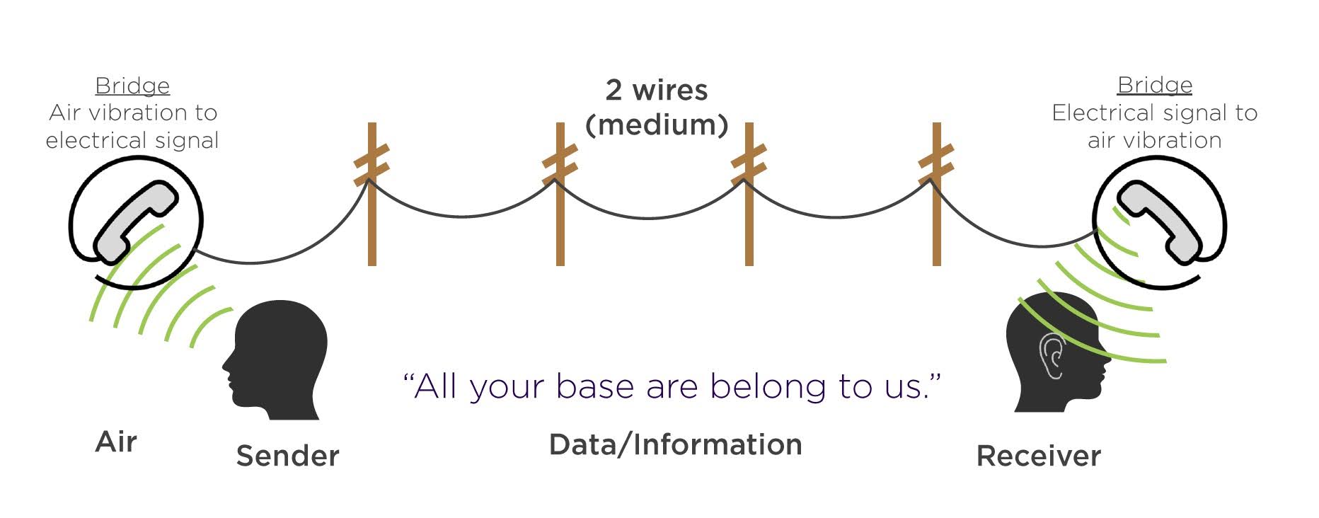
What does that mean? Well, let’s take a look at something that’s very common in our day‑to‑day life, and that’s using a telephone. Using a telephone is kind of like data networking, right? You have information in your head, you pick up the telephone, you dial your buddy, and you can tell your buddy the information that you have in your head, right? Or maybe you’re calling up customer service to either add services or cancel services. Either way, you have information that you’re trying to transfer. We have a sender and a receiver of the message. The message that we’re going to send, well, where does that come from? Well, the sender is going to conceive of something to say, in this case, “All your base are belonged to us,” which is broken English from a 1992 ported video game called Mega Drive. It’s become a popular MEME on the internet today, and I just picked it because it’s kind of silly here. “All your base are belonged to us” is the message we’re going to send. That message is in English, not great English, but it’s in English, the sender conceives of the message in English. Well, in order for the sender to get the message to the receiver at all, he needs some way of getting that message out of his brain and into the world around us. The way we do this, one of the mechanisms the sender has is to actually talk. The sender is going to use air and his vocal cords to vibrate the air, and in a way that allows this message, “All your base are belong to us,” to be transferred through the air. The sender’s vibrating the air with this message that he’s sending. When that message reaches the telephone, something called a bridge comes in play. Now the bridge is the microphone on the telephone, and this microphone, all it does is it’s a membrane, it’s a very thin membrane that vibrates with the air, there’s a small magnet attached to that membrane, and that magnet moves past some coiled up wires. Whenever you have a magnet and you move it past coiled up wires, you create an electrical signal. This is Alexander Graham Bell’s design, still the same one we use today, this bridge, this microphone, is going to take that air vibration and it’s going to convert it into an electrical signal that can be sent over two wires. These two wires, in this case, is called our medium. The medium for the vibrations was the air, the medium for the electrical signals is these two wires. When the electrical signal reaches the other end of the line, the receiver’s phone, what happens then is the electrical pulse is sent around a coil of wires, which is near a magnet attached to a membrane. Now you have the electrical signal causing the magnet to vibrate, which causes the membrane to vibrate, which produces a vibration in the air, exactly the same as the sender had originally sent. Now our receiver can hear the message, “All your base are belonged to us.” Now that was a pretty detailed and sophisticated explanation of how a message is moving from one side to the other, and in all honesty, if I was getting into deep, deep technical engineering‑level understanding of this, I missed all kinds of stuff that was happening in this process. But I wanted to keep it simple so that we could see a couple things happening here so that we can go model this conversation into some steps that can be a little bit more universal for us that we can apply in lots of circumstances.

Modeling Systems

The system that I’d like to create here, this model that I’d like to create to describe what happened, we’re just going to create four layers of this model. The top layer is the concept, then the language, then the link, and then physical. Now these words don’t necessarily have to have any meaning other than to generally describe possibly what’s happening. Sometimes they do a good job of it, sometimes not so much.

Let’s take a look. The concept here, this is the message, this is “All your base are belonged to us,” right? This currently exists in our sender’s head, and the sender is going to communicate that message in English. We have this model here where we have a message, and the message is going to be communicated in English. Well, we need a way to get that English language out into the real world, in this case we’re going to use some vibrations of air. Here air is our physical medium, and the way that we’re going to send the message across that air is through a vibration.

What I’ve done is I’ve broken down each component to fit into a different portion of the layers here. If I take a look then at what happens after the microphone is involved, our model still applies here because this time the microphone is going to use copper wires as the physical medium to transfer the information, but it’s not going to use vibration, rather, it’s going to use an electrical pulse or an electrical signal. Now at this point, we can’t really extract that to English and the message unless we convert that electrical pulse into something we can understand. And this is where now the speaker comes in where the speaker now takes that electrical pulse on the copper wire and allows it to be a vibration of the air. That vibration of the air then can be understood as English, and then that English can be constructed into the message that was originally sent. Here we have a case where we sent the original message, it was in English, we vibrated the air, it got converted to an electrical pulse over copper wire, converted back to an air vibration where our receiver could then listen to the message in English. Are there other ways to model this? Absolutely. Is this the best way to model this? Probably not. What I wanted to introduce, though, is that we can break apart communication systems into individual components. It’s not always going to feel user friendly, and it’s not always going to make a lot of sense until you start working with networking at a deeper and deeper level throughout your career.

Let’s wrap up this modeling systems here. We’re going to come back in the next chapter and talk about the OSI model, and I’ll explain how this OSI model kind of relates to the model that I’m talking about here.

Summary

Let’s wrap up this chapter. In this chapter, what we took a look at was, what is networking? Basically, saw that it’s just moving some data from one point to another. I took you through a general overview of understanding networking concepts so that you understand that even though networking is moving data from one place to another, there are lots of pieces involved, and there’s lots of interconnection between those pieces. We took a look at how we could model network communication to hopefully organize and better understand and later troubleshoot the protocols that are in data networking. We didn’t really get into any specifics other than the telephone call. I hope you enjoyed this chapter. Let’s jump into some real content and move into explaining the OSI model and how we’re going to use it throughout this article.

The OSI Model

Introduction

This the second chapter of the Networking Concepts article. This time we’re going to talk about the OSI model, or the Open Systems Interconnect model. Our goals this chapter is to introduce this model of networking. We’re going to briefly talk about how we modeled the phone call in the first chapter of this article, and then we’re going to go on and actually take a real networking example and use the OSI model to categorize all the different processes that are happening when we are using the internet.

OSI Model: Physical Layer

Let’s start off with the OSI model here. The OSI model, OSI stands for Open Systems Interconnect. This was developed in the early 70s. Some of the layers of this model are a bit antiquated, and I’ll let you know which ones those are. But for the most part, this is one of the most important things we can learn in data networking. Remember this from the previous chapter where we had a sender and a receiver. We were making a telephone call, and we broke that telephone call down into this model of concept, language, link, and physical. And we found out that we took this message, all your base is belonged to us, which is an English message. We converted that into a vibration over the air, which you had a microphone, which converted it into an electric pulse over a copper wire, which had a speaker, which converted it into a vibration of air again, which then our receiver could then understand some English words that all came together as, all your base is belong to us. Well, let’s look at how that happens in data networking.

To do that, what I want to do is I want to set up a network that you probably are familiar with. You’re most likely using some kind of computing device right now to watch video. On your computer, right, you have this video up on your screen, so let’s take a look at all the components involved in getting that message from the server over to your workstation. Your workstation is most likely connected to some kind of router. Here I have drawn a wireless router. The wireless router could have a physical connection where we can actually just plug in a wire, like might be the case where if you’re in an office, or maybe if you’re at home, you’re sitting using your laptop or your tablet, and you’re using a wireless connection to connect it. Either way, there is either a wired or wireless connection between your PC and some type of router that allows you to connect to the internet. Now the router that connects you to the internet doesn’t actually directly connect you to the internet, typically. If you’re at home, you might have an internet connection through an internet service provider. In my home, I use a cable TV service provider for my internet connection. I have something called a cable modem, which is that light blue device that I just plopped in the network that’s sitting in between the wireless router and the internet. Well, out on the internet then, there’s a whole bunch of servers connected. One of those servers is the xxx.com server, where you can browse to get the video content that we’re currently watching. I’m going to switch that connection from wireless to wired just to make the conversation a little bit cleaner here when we’re talking about the OSI model. Now, we’re not going to understand everything about networking if we understand the OSI model. However, if we understand some of the components of this model early on in our learning, we’re going to find out that we have a really great tool to categorize all of the little microevents that are happening when we’re moving traffic from one device to another. Let’s say that I want to go to the website. On my PC I type into my web browser www.xxx.com. That sends a message across the internet to the server. The server then pulls up the web page that I want to see, and it transfers it then over to my workstation were then I can view the content at xxx.com. Well, let’s take a look at all of the components that allow that to happen. First off, we have these cables, right? We have these wires that connect our computer to the router, our router to our cable modem, the cable modem out to the internet, and something is connecting our internet to the server over at xxx. There’s a bunch of cables in the internet as well. Some of them are wireless cables on the internet. Some of our point‑to‑point connections that we have on the internet that make it work are actually wireless, just like we have wireless networks in our own home or in businesses, or pretty much everywhere you go. The internet is composed of cables and some wireless connections as well. Well, if we’re more specific about those cables, not all those cables that we’re using are identical. As a matter of fact, the cables that we’re using in our home network or in our business network to connect PCs to the router or to the switch, or to connect to our cable modem, those are typically called twisted pair cables. And it’s a bunch of copper cables that are twisted together in a peculiar way to make the communication more efficient. We’re going to learn about twisted pair cables in another section of the net+ training. For now, just understand that there’s a cable type called twisted pair. Additionally, we might use twisted pair to connect the server to whatever devices it’s connected to get it to the internet. That may be fiber optic as well. It could also be some type of proprietary copper cabling. But for the most part in networking, right now we’re using twisted pair cabling when. We connect our cable modem though to our cable internet service provider, typically we’re using some type of coax cable here, which is a different type of cable than twisted pair. When we get out onto the internet, we’re going to find all kinds of different cables. Most of them are going to be fiber optic, which are glass. Some of them are going to be wireless. We’re going to have some copper in there as well. Some of that might be some proprietary copper cabling, and some of it might just be good old twisted pair cabling. On the Internet itself, we’re going to have all different kinds of cables that connect all the devices together to make everything work. All of these cables that we use in the protocols that define how those cables are constructed are physical layer protocols, all right? Twisted pair cabling involves a very precise protocol to understand how to construct it. You just can’t take a bunch of wires and slap them together and make a twisted pair cable. Same thing with coax. Same thing with fiber optics. And when we’re talking about wireless, this is especially true because we’re not really using physical wires, but we’re using the electromagnetic spectrum in order to transfer information. The physical layer is what we’re using here to connect all of our devices together. Let’s move on.

OSI Model: Data Link Layer

After the physical layer here, what we need is we need some protocols involved to move traffic from one end of the cable to the other end of the cable. We end up having these many network segments in here. A network segment is going to be a collection of network devices that all operate in the same space with the same protocol. Here there is a connection between our PC and our router. There’s another connection between the router and the cable modem, another one between the cable modem and the internet, another one between the server and some devices on the internet, and then the internet itself is full of all kinds of these little network segments that allow us to transfer data from one place to the other. Now, in each one of these circles, a specific network protocol is being used to manage and transfer the data. All right, if we look at what those are, most of them are Ethernet, all right? And this could be wired Ethernet, like I’ve drawn here, or it could be wireless Ethernet. But the protocol we’re using here is Ethernet in order to get messages from our device to the router, from the router to the cable modem, from the server out to some device that’s connected to the internet. If we take a look at that connection between the cable modem and our cable internet service provider, that’s using protocol DOCSIS 3. DOCSIS stands for Data Over Cable Service Interface Specification. DOCSIS, right? It’s a big, big mouthful, but all we have to know is that the protocol used here is DOCSIS. That’s what’s being used by our cable ISPs out there in the world. If we take a look at what’s happening on the internet, you would think that there would be all kinds of specialty protocols being used here, but really not. The internet is mainly Ethernet, and the reason for that is Ethernet is one of the few technologies nowadays that lets us get extremely high‑speed communication. When Ethernet first came out, it could only operate at 10 Mbps. Soon after, it went up to 100, then 1000 Mbps, or a gigabit per second. Shortly after that, we got up to 10 gig, 40 gig. Now we’re at 100 gig Ethernet, some of the internet service providers out there are actually having 100 gig Ethernet connections that connect one ISP to another ISP to allow for extremely fast and efficient internet communication. There are some other protocols out there like ATM or maybe SONET that are used as well, but primarily we’re using Ethernet here on the internet. When we look at all these protocols that connect the devices to other devices directly, the protocols we use here, like Ethernet, are part of the data link layer. The data link layer is going to be a place where we move traffic from one device to another device. It’s very small, short, little hops that we’re making here with the data link layer. Let’s keep moving on.

OSI Model: Network Layer

As I just said, the data link layer is responsible for moving traffic within these blue circles I’ve drawn here. I have some orange arrows drawn in there, and what I’m trying to say is that the data link layer moves traffic within that circle. The protocols there only do that, right? Ethernet can only move traffic from my maroon‑colored PC to the purple‑colored router. And then it can do it again from the purple‑colored router to the modem, and then from the modem out to some device on the internet, and then all within the internet, right? It can only do this communication between these short hops, but when we’re trying to communicate on the internet, that’s not going to work. Sometimes what we need is we need to be able to communicate from our PC out to, you know, the cable modem. Or maybe some communication needs to happen in the internet. Or more importantly, we need to communicate from our PC all the way to the server and back again so that we can get this video we’re watching. At this next layer of the OSI model, what we’re doing here is we’re going to use something called IP addressing to allow us to send messages across longer distances on our network. You might think of IP addresses kind of like your home address, right? Your home address has a street number, a street name, a city, a state, and a zip code, and all of those get more specific as to where you live, right? You may even put the country on a letter that you’re addressing. I live in the United States, right, so you’d put USA. I live in the state of Wisconsin, which is a smaller area within the USA. And then I live in a city called Madison, which is even a smaller area within Wisconsin, right? And then I live in a specific zip code within the city of Madison, which is a small area within Madison. Then I live on a specific street, which is even smaller. And then I have a specific house number, which gets me exactly to where I live. IP addressing works in a very similar way. It provides a unique address for all the devices on the internet, and that way, in addition to the IP addressing, we have IP routing, which allows us to send messages from one unique address on the internet to any other unique address on the internet. The way we’re doing this is the IP addressing allows us that end‑to‑end communication, whereas those data link layer protocols, like Ethernet, allowed us to communicate from one device to the next device. Ethernet and IP addressing and IP routing work very closely together to get messages from one device on the network all the way to the other side of your network. This is called the network layer. The network layer is where IP addresses and IP routing happen, and this is layer three of the OSI model.

OSI Model: Transport Layer

At the next layer of the OSI model here, what we need to do is actually, before we can have the server ever send us the website, or before we can even ask the server to send us the website, we have to set up some kind of session in between the client and the server, all right? This session is very similar to what we do when we make a telephone call, right? And this telephone call, one of the things I didn’t talk about with a telephone call is that I just can’t pick up the phone and start talking to my buddy. I can’t pick up my cell phone and say, all your base is belonged to us, and expect it to get to the person that I want it to. I have to set up a session between myself and the person that I’m making the phone call to, right? And the way that I would do that is I’d pick up my cell phone, I’d find the name of the person I’m trying to call, and I touch their name or maybe dial their phone number on my phone. I would then listen and wait for it to ring. I’d wait for my friend to answer. When they answered, then they would say, hello. I’d say, hello. And now I can send my message of, all your base are belong to us, or any other data that I want, right? At this point, it doesn’t matter what I say. I can just scream into the phone. But before I transfer that data, I have to go through that special process of dialing the phone number and going through the protocol to make the connection. The same thing happens here in data networking. At the fourth layer of the OSI model, we use something called Transmission Control Protocol, or TCP, to allow us to build this session between our client and the server so that we can say, hey, yeah, we built this session. Now I want to ask you for some data, which in this case is the website itself. This layer of the OSI model we call the transport layer, or layer four.

OSI Model: Application Layer

Now we’re going to find out here that I’m going to skip a couple layers. Don’t panic. I did this intentionally, all right? Let’s go on to the next section here and talk about the big intention of the internet, which is actually getting the website from the web server to our client. When I type into my browser www.xxx.com, that’s telling my browser, hey, I want to get that file over at xxx.com that has those videos that I want to watch on it. When I do that, this https//www.xxx.com is affiliated with the formatting of the website on the server itself. What I need is I need a protocol that allows me to transfer the website located on the server to my web browser located on my client. To do that, I use a protocol called Hypertext Transfer Protocol, or HTTP. Additionally, HTTPS for the encrypted version of it. Hypertext Transfer Protocol, what it does is web pages are written in a format called hypertext, and it’s a basic formatting of a text document to indicate instructions on how to present information in a web browser. This hypertext document, it’s literally a file, just like a Microsoft Word document. And we can transfer that file using HTTP or HTTPS for the encrypted version. HTTP here, the protocol that actually transfers the website from the server to the client, that is an application layer protocol, all right, and that is actually layer seven of the OSI model. Now, before I talk about layers five and six, which are not incredibly important in the land of modern networking, that’s my personal opinion, right, doesn’t mean that they’re not used, it means that they’re rarely used and they’re not incredibly valuable. But if we take a look at the OSI model without five and six for the moment, we have the physical layer, which is the cables. We have the data link layer, which allows one device to talk to the next device and the next device to talk for the next device. We have the network layer, which gives us an addressing scheme and a mechanism to move traffic from one side of the internet all the way to the other side of the internet. We have layer four, the transport layer, which lets us do the call setup. If we know the IP address of our destination, we can use a transport layer and TCP to say, hey, I want to transfer some data with you, right? And then we have the application layer, which will actually be responsible for moving the desired application from our server all the way to our client. These are the critical components of the OSI model that we need to understand in order to be successful network engineers.

OSI Model: Session and Presentation Layers

Let’s move on to these other two layers, layers five and six, which I always put a question mark by. In modern networks, I don’t believe they’re entirely important. I’ve had engineers argue this with me, and I support their argument in saying there are some protocols that do operate at layers five and six. When we are network engineers, though, and not developers, the distinction between five, six, and seven doesn’t become incredibly important. Let’s talk about layers five and six and see where they go. We’ll start here with layer six, the presentation layer. Now there was a time in networking when the presentation layer was super important, all right, and this is a time like in the early 70s. Now, when we are using our keyboard to type in something like all your base are belong to us, what happens here is we’re using a format called ASCII. And what ASCII does is it converts every letter, lowercase and uppercase, and all the symbols on our keyboard into a hexadecimal value. We’re going to talk about hexadecimal numbering systems a little bit later in this article, but for now, just know that it’s a way of counting that’s a little bit different than decimal, but effectively, it’s very similar. It just counts from 0 to 15, but it can’t count up to 15 with single values, it counts from 0 to 9, and then it adds A, B, C, D, E, and F in order to get up to 15. Like I said, we’ll talk more about that later on in this article when we talk about addressing. For now, just understand that ASCII is converting any letter on our keyboard to this hexadecimal value. Here A is 41. L is the number 6C in hexadecimal, which is actually a number. The space is 20. Y is 79. If I do this for all the rest of them, I get All your base are belong to us written in ASCII, looks exactly like this. And you can kind of see some resemblance here, right? It says 41 6c 6c 20 79. Well, that’s All-space y. In ASCII, we have this formatting. Well, ASCII was the open standard for encoding text. Well, back in the 70s, IBM was a massive hardware sales company, and IBM wanted to be different so that you had to buy their hardware and all their stuff to go along with it, they used a different encoding system called EBCDIC, all right? And EBCDIC did the identical thing as ASCII. It just did it completely differently, right? It assigned different hexadecimal values to different keyboard letters. Well, what the presentation layer did for us at one time is if you had a university organization running a non‑IBM system and you needed to network with a business system that was running IBM, you would need some protocol to translate the ASCII to EBCDIC, right, so that you could make this translation so that the IBM machine could understand the language and that the non‑IBM machine could understand the information being transferred. The presentation layer had some protocols that allowed this to happen. Occasionally, we had protocols that allowed for encryption to happen at the presentation layer, among other things, like formatting pictures and things like that. In modern networks, most of this formatting happens behind the scenes within applications completely outside of networking. EBCDIC, for the most part, is dead, and we don’t need it anymore. The presentation layer ends up being a somewhat antiquated protocol. The second layer that’s somewhat antiquated here is the session layer. There is a protocol called the Citrix ICA protocol that operates at the session layer. For the most part though, for a network engineer designing firewalls, networks, troubleshooting, and supporting, that ICA protocol, for the most part, we can see is also operating at the application layer. We just have it formally written in the specifications that ICA is a layer five protocol and not a layer seven protocol. You, as a network tech when you’re doing troubleshooting, aren’t going to have to concern yourself with understanding if it’s a layer five or a layer six issue. Most likely you’ll quickly be able to identify with lots of practice whether it’s a layer one, two, three, four, or seven issue on your network.

Summary

Let’s wrap up what we talked about here. We introduced the OSI model and talked a bit about how we use that modeling of the telephone call to set us up for this modeling of networking. And then we went through this practical example of getting the website from the server onto your client and all the different steps and the layers that have to go through in order to get that website to move from the server over to your workstation. The next section that we’re going to talk about here is going to be protocols, and there’s lots of protocols. What we’re going to do when we talk about those protocols is I’m going to be certain to always tell you precisely which layer of the OSI model that we are working with, all right? The OSI model, in my mind, is so important to organize things. When you are taking notes, you should always have a sketch of those seven layers written out so that while you’re listening to what I’m saying and watching on the screen, you can take notes about which protocol is happening at which layer. The sooner you can do this, the more effective network engineer you will be. I hope you enjoyed this chapter. Let’s jump into the next one where we talk about lots and lots of protocols.

Protocols and Port Numbers

Introduction

Our goals this chapter is to look at these application layer protocols. I’ve created some categories here that we don’t really use in the real world for these protocols, but it will be useful as we make our way through this chapter so that we can see some similarities in the protocols that we’re working with. We’re going to start by looking at data transfer protocols. We’ll then move on to authentication protocols, network service protocols, network management protocols, and some audio/visual protocols.

Transferring Data: HTTP or HTTPs

As a reminder, here we are using the OSI model throughout this entire series. We’re going to categorize nearly everything that we talk about into one of these seven layers. Right now, we are specifically talking about layer 7, the application layer. We’re going to start off with a very common use of application layer protocols and data networking, and that’s transferring data. And as a matter of fact, that’s typically all we ever want to do in data networking is transfer data from one place to another. As a matter of fact, in order to get to this video, you most likely used a web browser, browsed to xxx.com in order to get to the video. And in order to do that, the application layer protocol we’re using here is HTTP or HTTPS. This stands for Hypertext Transfer Protocol or Hypertext Transfer Protocol Secure. The secure version is encrypted, meaning that we’re going to encrypt all the data as we send it from the client to the server. Now as I say that, client and server here become incredibly important with application layer protocols. Nearly all application layer protocols use this model of having one device on the network being the client and the other device on the network being the server. Every once in a while, we may have a different setup than this, but for the most part, especially at all the protocols we’re going to look at today, client server is the model that we’re going to use. Now when we’re using HTTP or HTTPS to transfer a file, what we’re doing is we’re actually transferring a file in the format of hypertext. Alright, we can think of hypertext as a way of formatting a document in a way that’s readable by a web browser. You might think of this very similarly to maybe typing up a Microsoft Word document. And when we save the Word document, we save it as a .doc or a .docx file. Well, here we’re just saving the file in a specific format so that the web browser can open it. And the protocol itself that we’re using here is specifically designed to transfer these hypertext files used in websites. Now the mechanisms that are used to do this is on the client side. We’re going to use some client software to access the server. The client software you’re most likely very familiar with, this is either Google Chrome or Firefox, maybe Microsoft Edge, or Apple’s Safari browser. These are all web clients that support the use of HTTP or HTTPS.

On the server side now, the service side is also running some software. It’s running server software. For websites, we’re usually using Apache, which is an open‑source software that is a web server, which can run on either Linux or Windows. We have Nginx, which is used in very large website deployments and can be run on Unix. We have Microsoft’s Internet Information Services, or IIS, which can be run on Microsoft Systems. There’s several web server options out there that a server administrator can install in order to host a website on the internet. The whole purpose of the client server here is to have client software like a web browser and the web server software like Apache to work in conjunction with each other to transfer these hypertext documents in order to get the website from the server to the client so that you can watch this video.

Now I said we’re going to be exclusively talking about layer 7 protocols in this chapter, and we are; however, there’s something that’s really important to add onto this, and that’s that every single layer 7 protocol has a layer 4 component, and it’s called a port number. And the port number uniquely identifies the layer 7 protocol being used at layer 4. In this way, what we can do is we can use these port numbers to easily identify traffic at layer 4 so that computing systems understand how to interpret the traffic and what layer 7 protocol to send the particular messages to. For HTTP, by default, we have port 80, and for HTTPS, by default, we have port 443 as the transport layer protocols.

File Transfer: FTP, sFTP, TFTP, and SMB

Let’s move on to another way of transferring files here. This time we’re going to look at file transfer protocols. You could say, well, we just looked at a file transfer protocol, and you are correct. We looked at a protocol that transfers a hypertext document from a server to a client. The next one we’re going to look at actually allows us to transfer files from a client to a server or from a server to a client. We can do it in both directions here. And this protocol is either going to be FTP, sFTP, or TFTP. FTP is file transfer protocol. sFTP is secure file transfer protocol, and TFTP is trivial file transfer protocol. Let’s take a moment to identify each one of these. FTP and sFTP are pretty similar to one another. These protocols are going to transfer files from one device to the other and there is client and server software specifically designed to do this. Trivial file transfer protocol works a little bit differently. It’s really meant for sending tiny files between two devices or to have simple setups where you can transfer a file quickly without having to worry about authentication or having lots of issues with firewalls causing your traffic to be knocked down. FTP and sFTP typically require both the user’s name and a password in order to transfer these files. TFTP does not require this. SFTP specifically here is going to encrypt the traffic. Typically, whenever we see an s along with some protocol, that means that it is a secure protocol, especially if it’s written as a lowercase s like I’ve shown it here for sFTP. Now FTP uses some unusual port numbers here. FTP is going to use both ports 20 and 21. One is used for authentication. The other one is used for transferring information. Port 22 is used for sFTP. The reason for that is that poor 22 is actually the port number for another protocol we’re going to look at called secure shell, or SSH. And what happens here is we actually take the FTP protocol, and we put it inside of an SSH session which allows us to encrypt the traffic and is why the port numbers are the same for both sFTP and SSH. TFTP uses port number 69. Let’s move on to another protocol here, which we can add on to this. If we’re using Microsoft systems or even Linux systems, for that matter, we can use another protocol called SMB, which stands for server message block. And you’re probably familiar with this. If you work in an enterprise network or even in a small network, you probably have mounted on your desktop of your computer some type of network drive, some network file share where you browse to this network file share, and it gets you to a server where you can access files there that everybody else in the network can access. You can either put files there from your client, and you can put them up on the server. Or you can copy files from the server down to your client. Most likely you’re using SMB in order to accomplish this. We have numerous ways of transferring files between a client and a server. Probably the one used most often in an enterprise network, especially if you are a general end user, is SMB. If you are an administrator of servers, you’ll probably be using FTP, sFTP, and TFTP as often as you use SMB.

Demo: Examine FTP and SMB Operation

Let’s do a demonstration here and take a look briefly at both FTP and SMB operation on a desktop. What we’re looking at here is a Windows 10 workstation, and I’d like to show you two separate things. The first one that I’d like to show you is SMB, or Server Message Block. It’s what we use to mount a drive on a workstation, like I have here. What I can do is I can open up File Explorer. If I go down to Network, what I can do is right‑click on the word Network, and it’s going to say Map network drive. What I can do is map a network drive. It’s going to ask me to choose a letter, and then it’s going to ask me for a path to the server that I’m trying to connect to, and it gives me an example there. It says, use \\server name \share. What I want to do is I can put in \\. I have a server on my network that I call the tardis, or just tardis, and there’s a folder on there called demo, where I have some demonstration documents specifically for this. We’ll click to Finish here. It’s going to ask for my username and password on the tardis server. And then what will happen is it will map the demo folder onto my workstation. And I have two files in there. I have this router blue file, which is just a blue router drawing, and I have a switch in here, which is just an image of a network switch, or at least the icon for a network switch. Those two files are in that folder. If I want, I can add files to that folder. Let’s say I go to my Documents folder here. I can take this export, I’m not sure what that file is, it’s some HTML document, and all I have to do is just drag it over to the drive here, the demo drive, and now the export document is now in the Y drive on the tardis server. That’s using SMB to transfer some files. It’s using those mapped drives on our workstation. Another way we can do this is using FTP. All right, I have an FTP server set up elsewhere on my network, one of the ways I can get to an FTP server is by opening up Google Chrome, or any other web browser that I choose here. What I could do is then I type in the IP address of my FTP server. Except this time, instead of typing in http as the protocol in front of my server’s address, I’m going to type in ftp here. My server is at 10.128.50.16 We’ll hit Enter here. It should ask me for a username and password. Looks like it saved my credentials from when I was testing this. Username is xxx here, we’ll log in. And now what I see is I see a folder in my browser here with some files in it. One of those files is this testdoc.txt. I can click on that to open it up, and it should show me what’s in there. Can we download this, save link as something? Testdoc, we’ll save it to Downloads. If I open that up now, here it is, FTP Test File for Demo. All right, but what we can’t do with this is we can’t easily upload a file into this, what we need to do is instead we need an FTP client. All right, we can use our web browser as an FTP client, but it’s a little bit easier if we use an FTP client directly. Now, there’s an FTP client out there from Mozilla, who makes FireFox, and it’s called FileZilla. If I scroll down here and find my FileZilla FTP Client and open that up, what’s going to happen here is on the left‑hand side of my screen, it’s going to show me all of the documents on my local workstation. If I click on Downloads, we’ll see here that there is that test document that I just downloaded from the FTP server directly. What I can do here now is I can go in and put a host name in or an IP address, here the address is 10.128.50.116, my username is xxx, and the password I’ll put in, and we hit Quickconnect. And what that will do now is it’ll connect to my FTP server. This top window here says the status, it gives me a log message of what’s happening. It says, oh, I’m trying to connect here to the FTP server. It’s established, insecure server, I’m logged in, and it’s going to retrieve the directory listing. And here it is, over on the right‑hand side of my screen. If I go over into Files, there’s the test document that I downloaded. If I want now, I can go into another folder here on my workstation, and I could actually move another document if I wanted. Maybe I go to Documents here, and in my Documents folder maybe I try to move that export.html file again, move that over here to the place where the test document file is. Tells me that it successfully transferred the file. Now the file is located on my FTP server. I moved it from my client, which is the files on the left, to the server, which is the files on the right. If I go back to my Chrome browser here and refresh this window, we should see two documents in here now. One of them is the test document. The other one is that export.html. Here’s how FTP can operate on your workstation. Let’s move on to keep talking about more application layer protocols.

Email: POP3, IMAP, and SMTP

The next set of protocols that I’d like to take a look at here is email. Now email is specifically designed for transferring files. We’re transferring files that are actually in the format of these email documents. For email we have three protocols we use. Two of them are used by a client to retrieve mail from a server. POP and IMAP are explicitly used to take email messages that live currently on a server, maybe Gmail or maybe your company’s email server, and they’re used to transfer those email messages over to your client, some type of mail client that resides on your workstation. SMTP, however, is Simple Mail Transfer Protocol. This protocol takes a message that you create on a client email application, and it uses it then to send that email to an SMTP server, who will then forward it to whoever you’re trying to email. All right, we type an email up in our email client. SMTP is then used to forward the email to the server. The server then figures out how to get the message to the recipient that you intended. POP stands for Post Office Protocol. We’re using version 3 there. IMAP is Internet Message Access Protocol, and then, like I said, SMTP is Simple Mail Transfer Protocol. All these protocols work either in unencrypted or encrypted modes. We don’t add the s typically to these. Sometimes we will. But for the most part, we’re just identifying it with the port number itself to determine whether it’s encrypted or not. Here with POP3, for unencrypted traffic we’ll use port 110. For encrypted traffic we’ll use port 995. IMAP, we’re going to use port 143 for the unencrypted traffic, port 993 for encrypted traffic, and for SMTP, we’re going to use port 25 for unencrypted and 465 for encrypted.

Demo: Examine POP3, IMAP, and SMTP

Let’s do a demonstration then and take a look at the settings where we can see POP3, IMAP, and SMTP in an email client. I’m back in my Windows 10 desktop and I’ve installed another application from Mozilla. Mozilla, remember, makes FireFox, they also make a program called Thunderbird, which is their email client. I’m going to open this up and we’re going to add an account here to my email client. We have to go through some trickery here. Mozilla wants us to get an email account from gandi.net, I’m not sure what that is, I’m going to skip this and use my existing email address. Now most email clients, most modern email clients like this one are going to automatically try to configure all of the email settings for you. As a non‑network techy, you don’t have to worry about knowing what POP3 and IMAP and SMTP are, you can just plug in your username and password and it automatically configures it. Now, if you were configuring email clients 15 years ago, this wouldn’t have been an option for you, you would have had to put in your name here, I’ll put my name in. I’m going to make up on email address, I’ll say [email protected]. Since it has the .local, that means it’s definitely not on the public internet, and I’m just going to put a password in here, and we’ll hit Continue. Now it’s going to try to automatically configure this. I’m just going to go straight to the Manual Configuration button, which brings me to the information that I want to show you. And that is that if we look at our incoming mail, remember, the mail client I said is going to use either POP3 or IMAP to get mail from a server and pull it down to the client so that’s going to take incoming mail, mail coming in from the server, right? And we can use IMAP here. And if I drop that down, I can also choose POP3. We’ll start with POP3 here, it’s going to ask for the server name of the email server. It’s going to ask for the port number, and here it’s saying it’s going to automatically use the port number, but if we drop that down, we see that it can either use port 110 or port 995. If we look at our IMAP configuration, our ports here are either 143 or 993. SSL is our encryption and then we have authentication as well. Right now, that’s set to auto detect and that’s fine for these purposes where I’m just talking about where these configuration parameters exist within an email client. Now our outgoing server is SMTP. We don’t get an option of which protocol to use there. We can only use SMTP. And if we look at the port number that’s assigned there, we have 3 of possibilities here, 587 is sometimes used for encrypted SMTP traffic, we have port 25, and then we also have port 465. Here is the settings directly within an email client, where you can see IMAP, POP3, and SMTP options available for you. Let’s go back and keep looking at those application layer protocols we’ve been talking about.

Authentication: LDAP and LDAPs, and Network Services: DHCP

Let’s move on and talk about authentication. Now, there are some very specific authentication protocols used specifically with Microsoft’s Active Directory network environment. If you’re working in an enterprise organization, chances are, when you log into your workstation, you are using LDAP or LDAPs in order to communicate with server to authenticate you to the network, bring down all of your map network drives and get you your settings. LDAP stands for Lightweight Directory Access Protocol. And here we will be using, on the client side, we’d be using something like Windows 10, and on the server side, you would use something like Microsoft’s Active Directory, which is part of their server line of products. And it allows you to automatically push policies and automatically configure Windows clients from that central server. The way that that works is when we log in, we’re going to put a username and password into our client. That username and password is sent to the Active Directory server. The Active Directory server looks up in its database, determines whether or not you have legitimate credentials. If you have legitimate credentials, what’ll happen is LDAP will then send a token back to the client and say, yes, this user is authenticated for the network access, allow the user onto his workstation. The port numbers we used here, LDAP uses port 389. LDAPs, for the encrypted version, uses port 636. In all modern implementations of this, we should definitely be using LDAPs on port 636 Let’s talk about network services. Here we are starting to move into cases where we’re not actually transferring files. Rather, now we’re transferring data, or little bits of information that allow the network to work properly. One of these is Dynamic Host Configuration Protocol, or DHCP. The way this works is that when we plug into our network, even our home network, there is a DHCP server on our home network. Typically, in your home network, that DHCP server is your wireless access point, the thing that connects your network, or all your computers, to your cable modem router or your DSL router or maybe your satellite router, whatever Internet connection service you have in your home. And what it does then is it automatically hands out IP addresses to any device that’s connected. The way this works, when we turn on our workstation, what’ll happen is our workstation is going to send a message to the DHCP server saying, hey, I just came on the network and I don’t have an IP address. And then what will happen is the server will say, well here’s an IP address, subnet mask, default gateway, a DNS server and maybe some other information you can use to automatically configure yourself on the network. All right, and this way, what we don’t need to do, then, is have an administrator come by and configure your PC to have specific information statically configured and permanently configured on your workstation. Now this becomes really valuable when you have a mobile device, like a tablet or a laptop or a smartphone, when you’re moving from network to network to network quite a bit, we don’t want to have a static configuration that’s unchanging on our devices, because then when we moved to a new network, we’d have to actually go and manually change it to the new settings, which we may not know what those are. With DHCP, what that allows us to do is when we do come into a new network, it says, hey, automatically tell me the information that I need to know to connect to this network and allow me access to the resources I need.

Demo: IP Configuration via DHCP

Let’s take a look at the IP configuration with DHCP on our workstation. Now I’m back on my Windows 10 workstation, and what I want to do is open up a command prompt. Now Command Prompt we can get to many ways. I have a shortcut on my desktop here. If I search for it, I can type in cmd, and that will bring up Command Prompt. All right, and in the Command Prompt here, I can do a couple things. I can type in the command ipconfig. And what that’ll do is, it’ll show me the IP address and other information that is currently configured on my workstation. This includes my IP address itself, the subnet mask, and the default gateway. In the upcoming chapters, we’re going to talk a lot about IP addresses and subnet masks. Until then, understand that each device on our network must have an IP address in order to communicate with the rest of the devices on the network. I can actually manipulate this information a bit on my workstation. If I issue the command ipconfig /release what that will do is, it will release the DHCP lease of the IP address. The way DHCP is working here is, we’re actually just temporarily borrowing an IP address to use while we’re connected to the network. Even if we’re always on the same network, this address is kind of temporary. We can release that address, and what happens then is, when I issue ipconfig now, there is no IP address on my PC. If I say ipconfig /renew, what that will do is, it’ll ask the DHCP server to give me a new IP address, or maybe not even a new IP address, but give me an IP address. Typically, what will happen is, it will give me that last IP address that I had. Here I’ve got an IP address now by using the ipconfig /renew option. When you’re working with this, if you issue ipconfig /release and then renew and you don’t get an IP address, usually that means there’s some technical problem with your network that needs to be fixed. We’ll get into more of that type of work in a future article, when we specifically talk about troubleshooting networks. For now, you have a general idea of what our DHCP server is doing for us. It’s automatically configuring this IP address for us on our workstation.

Domain Name System (DNS)

Let’s keep moving on. Next protocol we’re going to talk about here is domain name system, or DNS. DNS is an incredibly critical protocol in data networking, because what it does for us is it allows us to use simple names to communicate with devices on the internet. Every device on the internet gets an IP address. Here on my client, I’ve given a fake IP address of 203.0.113.55. I see that’s fake because it’s actually not an IP address that’s routable on the public internet, but we’re going to use it here just for this example. Google.com has an IP address of 216.58.216.206. And then there’s a DNS server on the internet of 8.8.8.8. Those are real IP addresses, both google.com and the DNS server. Those are real IP addresses of, actually, Google and Google’s DNS server on the public internet. What will happen is when I type into my browser www.google.com, what’ll happen is my workstation is going to send a message to the DNS server that’s configured on my client. My DNS client here is my work station itself. It sends the message to the server and says, Hey, what’s the IP address of google.com? The DNS server will respond then with the IP address of google.com. Then what I can do is I can say, Hey, google.com at 216.58.216.206, send me the website. And it’ll grab the website together, and it’ll get the website, and it will send it over to my workstation. Any time we’re using the internet to browse to any website that we go to, before we go to that website, we are first making a detour to a DNS server to find out what the IP address is of that particular server. Every single server on the internet we communicate with must have a public IP address, or we won’t be able to communicate with it.

Demo: Examine DNS Using nslookup

Let’s do a demonstration here where we can examine how DNS works using a command called nslookup. I’m back on my Windows 10 workstation, I’m going to type cmd to get to the command prompt again. And this time, instead of using the ipconfig command, I’m going to use the nslookup command. Before I use that nslookup command, though, I’m going to go back to my ipconfig command and I’m going to put /all after the command. What that’ll do is it’ll show me my entire IP configuration including the configured DNS server. Now, the DNS server is typically automatically configured by DHCP. When I use the nslookup command to say find the IP address of google.com, what I would do is I type nslookup and then I type the URL of the site that I’m trying to find the IP address for. I do nslookup google.com, and it comes back and it gives me an IP address. Here, it’s saying it’s 172.217.4.78, it’s also giving me an IPv6 address here. We’re not ready for IPv6 addresses quite yet, but in a few chapters, I will explicitly talk about IPv6 addresses and how they work. For the time being, we only need to worry about our IP Version 4 address here. Now I’m going to clear the screen, cls. Another way we can use nslookup is to just type the command in and hit Enter, and what it will do is it’ll say, well, the default DNS server here is this device called router.doryhouse.local, which is actually my router in my house, has an IP address of 10.128.50.1. If I want, I can change the IP address of the server that I’m using to resolve the name into the IP address. If I say my server is at 8.8.8.8, now it says, okay, now my default server is google‑public‑dns‑a, right, and that’s Google’s public DNS server. Now I can type in an address like google.com or a name like google.com, it will tell me the address, it’s the same address that I saw before, maybe I want to do facebook.com,. it’ll tell me the IP address of Facebook there at 157.240.2.35, right? Any website that we want, xxx.com, it’ll tell us the IP addresses of the site that were visiting. Now here, xxx is showing three different IP addresses, and what this typically means is that xxx is hosted at more than one location, so that we can guarantee, as best as we can, that the website stays off and as much as possible. What it’ll do is it’ll sometimes return the IP address of 54.69.212.232 as the first IP address. Sometimes it’ll pick the 35. IP address, and sometimes it’ll pick this 52.88 IP address to be the primary IP address that your work station will use to contact xxx. The IP address that your workstation will use is typically going to be the first IP address in the list here. DNS, it’s specific purpose is to do these lookups of hostnames like xxx.com into an IP address that we can use to actually get to the website to get us the data.

Network Time Protocol (NTP)

Let’s move on to our next section here where we’re going to talk about Network Time Protocol. Now Network Time Protocol, or NTP, is a way that we can use a server, a Network Time Protocol server on our network, to automatically configure all of the times on our clients to be exactly the same. The way that works is a client on the network, which is usually configured with NTP right in the operating system itself, can send a message to the NTP server saying, hey, what time is it? And the server can reply what time it actually is; it’ll say, hey, it’s 3 p.m. Now the Network Time Protocol servers, these are oftentimes public servers run by the government, and the time that we use is not actually as simple as I said here; it’s 3 p.m. The time is a little bit more complicated than that, because there are time zones all over the world, and at any given moment, the way we record the time on a specific place on Earth is going to be different, right? The way we use that is we use coordinated universal time or UTC in order to fix this. And the UTC allows us to accommodate for the time zones. Now how this works is there is an imaginary line that goes from the North Pole to the South Pole of the Earth, and that imaginary line has a 0 marker as it passes through Greenwich, England. Alright? Greenwich, England is just a bit east of London, and that line is called the Prime Meridian. And the Prime Meridian, the time at the Prime Meridian at midnight is 0 hours, alright? It’s 0:00 hours at midnight on the Prime Meridian. Everything else is measured against this midnight time at the Prime Meridian. If I want to know what time it is in Chicago, whatever UTC time it is in Chicago, it’s going to be six hours before then. Now this is assuming that Daylight Savings Time is not applied, alright? Daylight Savings Time adds a whole other complication to this that we’re not going to get into in this article. But just understand that Chicago is six hours before Greenwich. If it is midnight in Greenwich, it’s 6 p.m. in Chicago. If we go a little bit further here, out in Utah, it’s an hour earlier than that. At midnight in Greenwich, it’s 5 p.m. in Utah. If we take a look at another area of the world here, let’s look at New Delhi. When it’s midnight in Greenwich, England, it’s actually 5:30 in the morning in New Delhi, alright? In New Delhi, India, they’re a half‑an‑hour difference from what it is in Greenwich, England, in addition to that extra five hours. Depending upon where we go on Earth, the UTC is going to be exactly the same number. We’re just going to add or subtract the correct number to UTC to get the time in our local area.

Network Management: Telnet and SSH

Let’s look at in the next section of application layer protocols here, network management. In network management protocols, we have two big ones here, Telnet and Secure Shell, or SSH. I mentioned SSH before, when we were talking about FTP, and SSH is encrypted, whereas Telnet is clear text. SSH can be used to do all kinds of nifty things, including accessing our devices remotely, as well as using it for something like a mechanism to encrypt FTP traffic. Telnet operates on port 23, SSH operates on port 22. When we are working in a network environment, our network administrator may need to communicate with several kinds of devices. Maybe they need to communicate with another server or a router or a switch. And in this case, the network administrator’s workstation is the client for either Telnet or SSH And the server, in this case, will either be the server that were trying to SSH to or the router or the switch. These devices will take on a role of server in order to allow that communication to happen. All right, that could even be something like a firewall that we add on. We might SSH or Telnet to a firewall.

Demo: Examine SSH Use

Let’s do a demonstration of SSH use here. I’m going to jump back to my workstation. I’m going to move to my workstation here, and I’ve downloaded an application called PuTTY. Now, PuTTY is a free, open-source tool, that is an SSH and Telnet client, among other things, but we primarily use this for SSH. What I can do here is I can put in an IP address of a device that I might want to SSH to on my network. I have a device, a router, I have at 10.50.128.117. If I hit Open, what that’ll do is it’ll open a session to that device. Maybe that device isn’t accessible here. Alright, well, let’s try that again. We’re going to close this window. Let’s send a ping message out first; ping 10.128.50.117, and I am getting a response from that. Let’s try our PuTTY session again here. We’ll open up PuTTY, and go to SSH 10.128.50.117. Here we go. It’s saying, hey, this is using an old algorithm that may not be super secure. I’m not too concerned about that, because this is all within my local network. I would never set up a router to use this less‑than‑ideal encryption algorithm that we’re using here. However, that’s all information for a much later date in your networking education. I’m going to log in here. I can log in as xxx, and what that does now is it gives me a command prompt for a different device on my network. Alright, I can issue commands here to show me different things on this router. Right now I’m connected to this device via SSH. This isn’t my local workstation. This is a remote access to another device using the SSH protocol. This SSH utility can be used all over the place, and it is used all over the place in order to configure networked devices, both servers as well as other hardware.

Simple Network Management Protocol (SNMP)

Another network management protocol we use here is something called Simple Network Management Protocol, or SNMP. SNMP, what it does is it uses an SNMP server to then collect information about SNMP clients or agents. And what will happen here is the SNMP server can send out a message and do something called walk the tree. And it sends out a message, and it says, hey, device, tell me everything that there is to know about you in SNMP land. And this could include the statuses of ports. Is the interface up or down? What’s the processor utilization of the device? What’s the temperature of the device? Are there any other issues or log messages that are important, right? We can go walk the tree, and it can give us all kinds of information about our devices, which will then report back and say, yep, here is all of my information. Add it to your database SNMP server. And then what that’ll let the network administrator do is browse to the SNMP server and view graphs and statistics about the performance of the devices on the network. Another thing that can happen is if a device on the network, something breaks on it, like our switch here started on fire, maybe it’s too hot, what it can do is it can send something called an SNMP trap to the SNMP server, which then allows the SNMP server to maybe add it to the database or maybe send out an alert to the network administrator that, hey, there’s a switch on fire some place in the building.

Remote Desktop Protocol (RDP) and Audio/Visual Protocol

Another utility that network administrators use often is something called Remote Desktop Protocol, or RDP. Remote Desktop Protocol here, what it allows us to do is if we’re sitting at our desk and we need to get access to the desktop of a server, RDP allows us to use an application called Remote Desktop to actually put the IP address of the server into that application and then it shares the screen of the server onto our workstation and allows us to remotely manage that device. RDP is going to use Port 3389 here. The last protocols we’re going to talk about are audiovisual protocols. One of them is going to be H.323 here. H.323 operates on Port 1720, sometimes 1721, and what it’s used for is audiovisual communication, typically used for videoconferencing. Here we have a group of people on the left that we can see on the monitor for the group of people on the right and vice versa. We see the group of people on the right on the monitor on the left, and what’s happening here is there’s a video conference happening. The video conference connects these two monitors and cameras together and allows for audiovisual communication to happen in between these two different presentation rooms. H.323 is our protocol to do that. Another one we can use typically more for voice over IP is called SIP, or Session Initiation Protocol. This is going to use either ports 5060 or 5061. And it’s used to help set up a voice call between the phone and the server, sometimes the server and the telephone company. SIP can be used in lots of different applications, but we typically find it used in our telephone communications when we’re using voice over IP communications in a network.

Summary

To wrap up what we’ve done here, we’ve looked at a lot of protocols. We took a look at data transfer protocols like HTTP and FTP. We looked at authentication protocols like LDAP, some network service protocols like DHCP and DNS, network management protocols like SSH and SNMP, and then some audiovisual protocols like SIP and H.323. I hope this chapter was useful for you. What we’re going to do in the next chapter is go through the Layer 4 protocols and eventually show how the Layer 4 and Layer 7 protocols are connected together.

TCP and UDP

Introduction

Our goals this chapter is to take a look at these two transport layer protocols. These are layer four protocols. The first one is Transmission Control Protocol, or TCP, and could easily be argued one of the most important protocols in data networking. The second one here is User Datagram Protocol, or UDP. As we make our way through this article, what we’re going to do is take a look at each of these protocols, we’ll take a look at port numbers as well, and then examine some protocol hierarchy and examine how application layer protocols relate to transport layer protocols, as well as network layer protocols.

Transmission Control Protocol

We take a look at our OSI model here. In the previous chapter, we looked exclusively at layer 7 protocols, that application layer. Now we’re moving down to the transport layer at layer 4. Remember, I said layer 5 and 6 are not used heavily in data networking, we’re going to skip over those, and go to some of the most important protocols in data networking, which are TCP and sometimes UDP.

Let’s start off by taking a look at this example we had here of transferring our website from the server to the client. Now in order to do that, we have to establish a session in between the client and the server, and that session essentially is a mechanism, so that we can say yes, I want to get some data from you, we’re going to set up this specialized communication session. And we’re going to use the protocol, Transmission Control Protocol, or TCP, to accomplish this. Now TCP behaves so similarly to something that we do regularly in our lives. Before I explain how TCP works, let’s take a look at this conversation on the telephone between Homer and Marge. Now, Homer has Marge’s phone number here, 867‑5309. For some reason, I think that’s phone number of somebody else, but regardless, what Homer needs to do in order to talk to Marge is he has to go through a specialized process. He cannot just pick up the phone and start talking to Marge. What Homer needs to do is he has to pick up the phone, he has to wait for a dial tone, after the dial tone comes, then he can dial the phone number. After the phone number is dialed, he’s going to wait for the phone to ring. After the phone rings, he’s going to wait for Marge to pick up the phone, and answer, and say hello. Once Marge says hello, Homer can say hello. At this point, we have established a session in between Homer and Marge. Before Homer can say anything to Marge about her blue hair or anything else she has going on, Homer must go through that exact process, or he won’t be able to talk to Marge. During the conversation, alright, when Homer is saying, hey, your hair looks pretty, Marge, Marge may hear that and say, oh, I see. Thank you, Homer. And Homer may acknowledge that by saying uh‑huh, I understand what you’re saying, Marge, right? Throughout the conversation, both Homer and Marge are giving these clues as to whether or not they received the message from the other party. In addition to this, maybe Homer or Marge didn’t get the message that was sent, or they didn’t get the entire message that was sent. Homer may say I don’t understand, or maybe Marge says you’re breaking up, meaning can you repeat what you just said because I didn’t hear what you were saying, something happened, right? We have these ways in our session of letting the other person know that we didn’t get the information they sent. Last, we have a protocol for ending the session. That can be anything from as nice as goodbye and then hanging up the phone, or it could be more abrupt, where maybe Marge gets angry at something Homer said and just hangs up the phone without even saying goodbye, right? These are all mechanisms to end the session between the two parties and prevent future communications. What do we have going on here? We have a specialized process to establish the session between the two people talking on the telephone. We have ways in the conversation of acknowledging that information was received or acknowledging that information was not received. And then last, we have a way of tearing down the session, whether that be a polite version of saying goodbye or something more abrupt of just hanging up the phone.

The 3-way Handshake

When we look at TCP, TCP does something called the 3‑way handshake, which is much like what we just did when Homer and Marge talked on the phone. Homer had to pick up that phone and dial the phone number, right? He had a pick up the phone, wait for the dial tone, dial the phone number. Here, once we know the web server’s IP address, we can send it a message called a SYN message or a synchronized message. That SYN message will then change a state on the devices to say that, hey, a SYN message was sent. We’re waiting for a reply now from the server. The server will then send a reply. Alright, on the server, as it sends the reply, it’s going to change its state to SYN‑RECEIVED, meaning that it has now sent a message to the client called a SYN‑ACK or an acknowledgment of the synchronization message. The client will then respond with a message saying ACK. We send this ACK message to the web server, and now, at both ends, we have a session established between the PC and the web server. SYN, SYN ACK, ACK. These are the three steps to establishing communication between a client and a web server or any server for that matter. Alright, let’s move on. Once we have the 3‑way handshake established, then we can use a protocol like HTTP or HTTPS to send another message to say, hey, send me the website, and then the server can reply and say, here’s the website. Now if you notice what happened here, this is much like what happened with our telephone call. We establish the phone call by dialing the phone and waiting for it to ring. In TCP, we did the 3‑way handshake, waiting for the SYN, SYN ACK, ACK messages to complete. Once that was done, the layer 4 protocol was complete. We didn’t use that anymore. Now we’re using a layer 7 protocol to say, hey, what’s the website? And then the web server is coming back and saying, here’s the website. We used the layer 4 to establish a session and layer 7 to actually transfer the website itself. During this conversation, if maybe the entire website didn’t get sent to the client, the client can then send a message back to the server saying, hey, I’m missing information. If the web server doesn’t fully get the entire request from the PC or maybe you’re entering a form and the web server doesn’t receive it all, the web server can send a message back to the PC saying, hey, send me more information. I didn’t get that last message. With TCP, we have a way of navigating the conversation to say yes, I heard what you said or no, I didn’t hear what you said. Please resend it.

The 4-way Disconnect

When we’re disconnecting, we can have a very graceful session disconnect like we did in our phone call by saying goodbye. Here we can have a four‑way disconnect where one device sends a FIN message for finish, another device sends a FIN‑ACK message saying, I got your FIN and here’s the acknowledgement for it. That device will then reply again with another FIN message. And then the Web server is going to finally respond with that FIN‑ACK message that says, yep finally, the conversation is closed. Now we may no longer send any HTTP requests. All right, the conversation is shut down. We’ve hung up the phone at this point. We can’t tell Marge any more information. Marge can tell us any information. FIN, FIN‑ACK, FIN, FIN‑ACK shuts down a session. Another way we can do this is we can very quickly end a session by sending a message called a reset. And a TCP reset is just basically like hanging up the phone. The Web server may say, hey, this conversation isn’t right, something’s wrong with it. It may send the reset. It may just say, okay, we’re done transferring the website and send a reset. There may be a device someplace in between the PC and the Web server, something like a firewall, that decides that the conversation isn’t good, and it shuts the conversation down with the reset. Reset is just like hanging up our phone. It shuts down the conversation and prevents further communication from occurring.

User Datagram Protocol (UDP)

TCP is a very reliable protocol, has mechanisms built in to verify that the data sent was received, has this nifty message of setting up a session between the endpoints, and has a nice way of ending the session. User Datagram Protocol is another transport layer protocol that operates a little bit differently. And here, when we have a client and a server, all we’re doing with UDP is we’re going to wrap up some application‑layer message like maybe DNS, and say, hey, send me the data, and then the server comes back and says, here is the data. Notice that we didn’t set up a three‑way handshake to get the data to transfer. There is no session set up. This is kind of just like opening your front door and shouting out to the world, hey, I need some information, and then hopefully one of your neighbors will open their door, and shout back, and say, hey, I have the information for you, right? This isn’t anything like making a phone call at all. This may be more like using maybe a walkie‑talkie, where we send a message out onto the walkie‑talkie system, maybe we address it to a certain person, but we don’t necessarily do the same thing we did into the telephone, right, where we picked up the phone, and dialed, and all that. With the walkie‑talkie, all we have to do is pick up the walkie‑talkie, push the button, and say, hey, I need some information from Bill, right, or hey, I need some information from Marge, and hopefully Marge will respond to us. In this case, we’re doing something similar. User Datagram Protocol, there’s no three‑way handshake, there’s no reliable communication, meaning that the message sent may or may not be received by the server, and we have no way of knowing that. There’s no sequence numbers or acknowledgement numbers here. Sequence numbers and acknowledgement numbers are used in TCP to verify that the data sent was received, there’s none of that in UDP. It’s very, very efficient for small data transfers. As we learned in the previous chapter, there’s a protocol called DNS, Domain Name System, and it’s used to resolve a host name like google.com into a usable IP address that can be put into an IP packet header. Well, the value of UDP here is that for a protocol like DNS, it’s just a simple message that we send to the server saying, hey, DNS server, what’s the IP address of google.com? That can easily be sent in just one single message to the server. The server can then respond to that message saying, yeah, I’ve got that. Here’s the reply to it, Google is at 8.8.8.8, or whatever other IP address it responds with. Because there’s such a small amount of data here, we don’t need to say SYN, SYN‑ACK, ACK, hey, what’s the IP address of Google? Here’s the IP address of Google, FIN, FIN‑ACK, FIN, FIN‑ACK, right? We don’t need all those messages to do this with DNS, we can use something like UDP to keep the process short and sweet.

Transport Layer Addressing: Port Numbers

Transport layer addressing. Let’s take a look at port numbers here. At the transport layer, we are using port numbers to identify typically an application layer protocol that’s being used. In TCP or UDP, there are always a source port number and a destination port number in our segment header. These port numbers are categorized into different areas. We have server port numbers, which are categorized into well-known and registered port numbers. And then there are client port numbers, which we call ephemeral port numbers. Ephemeral here literally means temporary. Temporary port numbers. Let’s take a look at what these are. Well-known port numbers are between 0 and 1023, registered port numbers are between 1024 and 49,151. And then our ephemeral port number range is from 49,152 to 65,535.

Typically, we’re going to see well known port numbers used as our destination port number when we’re communicating with a server. Let’s take a look at those. We’ve already seen some of these like HTTP, HTTPS, right? At 80 and 443. We’ve seen FTP operating on 20 and 21. SSH operates on 22, Telnet port 23. Our registered port numbers are going to be for custom applications, and they have both official and unofficial port numbers. In this registered port number range, you’re going to see some very unusual things, oftentimes proprietary protocols, like IBM has a bunch of proprietary protocols in there. H.323 has some protocols in there, like we saw. SIP also has protocols in there. There’s a protocol called RADIUS, which we use to authenticate, which has a port number in this registered port number range. We may see port numbers as a destination port in either the well-known or the registered port number range when we’re working with TCP or UDP.

When we’re using these transport layer protocols, or in this case TCP, for Telnet, what’s going to happen is when we send out our message, our SYN message, our SYN‑ACK message, our ACK message, and then every piece of communication between the PC and the router, in this case, what’s going to happen is the source port is going to come from the client, and that’s going to be in the ephemeral range. The destination port here is going to be whatever service were trying to access on the destination device, in this case, Telnet on port 23. In that TCP header, which is called our segment header, we’re going to include these source and destination port numbers.

Application Layer Protocol Dependency

Let’s wrap up this chapter by taking a look at the application layer protocol dependencies in each layer of the OSI model. If we start here with the protocols that we looked at in our OSI model, or at least some of them, these are the File Transfer Protocols we looked at, each one of these protocols has a port number assigned to it. Those layer 7 protocols have a layer 4 port number assigned. Those layer 4 port numbers are specifically assigned then to some layer 4 protocol, either TCP or UDP. What I’ve done here in this chart is I have mapped out which layer 7 protocol uses which layer 4 protocol. You can see that most of them are using TCP, HTTP, HTTPS, FTP, SFTP, SMB, POP3, IMAP, SMTP, and LDAP secure all must use TCP at the transport layer. LDAP can use TCP or UDP, depending upon how it’s configured, and TFTP, Trivial File Transfer Protocol, on Port 69 exclusively uses UDP. Now all of these protocols are going to use IP at the network layer. We have an application layer protocol. We have a transport layer protocol that that application layer protocol is assigned to. And then they’re all going to use IP at the network layer. If we take a look at the rest of the protocols that we looked at in the previous chapter, we see that Telnet, and SSH, and RDP all must use TCP. DNS, SIP, H.323, and SNMP can use either TCP or UDP, depending upon the way the protocol is configured at the application layer. And then DHCP and NTP exclusively use UDP at the transport layer. All of these protocols, again, are going to be wrapped up inside of IP at the network layer.

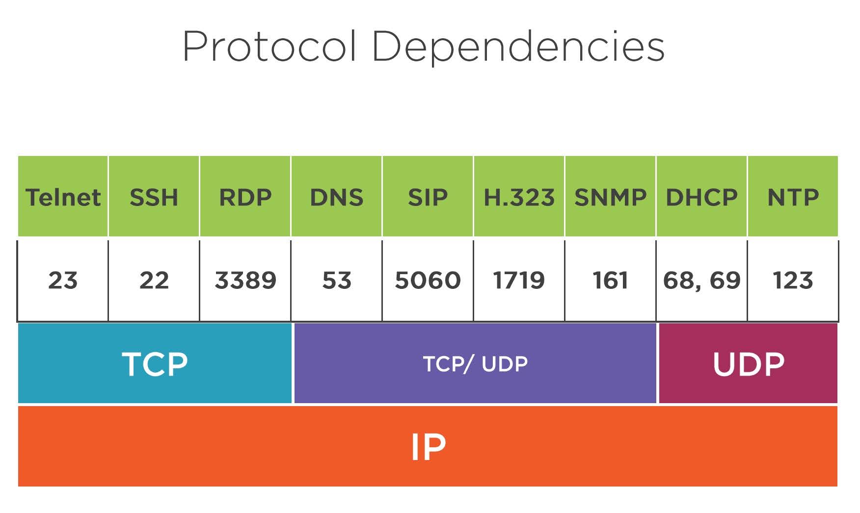
Summary

To wrap up what we’ve looked at here, we took a look at transport layer protocols, specifically TCP and UDP. And then we took a look at the port numbers, the protocol hierarchy, that each layer 7 protocol uses with each layer 4 protocol and saw that all of them use IP at the network layer. I hope you found this portion valuable. We’re going to move on to the next section where we start taking a look at the network layer in more detail and specifically focus on IP addressing.

Introduction to Binary and Hexadecimal

Introduction

In these next several chapters, what we’re going to do is take a look at network layer addressing, specifically IPv4 and IPv6 addressing. However, in order to understand what’s happening in those addressing schemes, we really need to understand what’s happening with binary and hexadecimal. We’re going to take this chapter here and learn how to convert from decimal to binary and from binary to decimal to hexadecimal. We’re going to introduce the need for binary here and explain a little bit about what happens. We’re going to review some primary school mathematics. Yeah, I know that sounds a little awful maybe, but I’m going to make it as easy as possible. We’re going to look at how we count in binary. We’re going to convert binary to decimal and decimal to binary. Last, we’re going to take a look at how hexadecimal fits into all of this and how useful it is in data networking, especially in IPv6 addressing.

Binary 101

Let’s get into binary 101. When we normally count, we’re counting in base 10. We normally don’t think about it because counting becomes such an important part of our life. The numbering system we use isn’t even paid attention to most of the time. We count in base 10 most likely because we have 10 fingers. Binary, on the other hand, were only counting with 2 values in the placeholders, either 1 or 0, on or off. In decimal we had 10 values, 0 through 9. In binary, we have 2, either 0 or 1. An example here, if we look at counting in decimal, we have to go all the way back to our grade school days, to primary school days, and remember these placeholders in the powers of 10. We start counting in the one’s placeholder with 0, then we count up to 1, 2, 3, 4, 5, 6, 7, 8, and 9. Right, when we get to 9, we run out of values to fill into our placeholders here. We have to add another place holder, the tens place holder. Then we can start counting in are one’s placeholder again, right? All the way from 1‑0, 10, all the way up to 99, when we reach 99 we’ve used up all of the values of 0 through 9, both the ones and the tens placeholder, we have to add another placeholder. This time we add the hundreds placeholder. After we count to 999 we add another place holder, the thousands then the ten thousands, then the hundred thousands, then the millions, then the ten millions, and so on. We count this way because of the 10 fingers on our hands, and it evolved into this decimal system of counting. When we’re working at a computer though, the computer can’t think in 0 through 9, it can only think in 1 or 0. When we’re counting in binary, we’re working in the powers of 2, not the powers of 10. When we start off counting in binary, we start counting just like we do in decimal. We start with 0 and then we count up to 1. But when we get to 1, we’re all out of values to fill up that one’s placeholder. We can’t count to 2, there is no number 2 that we can fill in the one’s placeholder in binary. What we have to do is we have to create a new placeholder. After 0, then 1, we create another place holder called the twos placeholder, and then we start counting. Here we have 0 0, 0 1, then we have to count to 1 0, right? We filled up all the values in the one’s placeholder with 1. The next value we have to put into the two’s placeholder, and then put a 0 in the 1’s. And then the last value here is 1 1. Well, this keeps going on and on, right? here, if I just take that same set of values here, and I add another placeholder, the fours placeholder, if I start counting here again, I still have 0 0 0 for 0, 0 0 1, 0 1 0, 0 1 1, and then, to get to the next value, our fourth value here, we have put a 1 in the fours placeholder and then put 0s in the twos and the ones placeholder. This pattern then keeps repeating. All right, we have 1 1 0 is the sixth placeholder here or the sixth value after 0, 1 1 1 is our seventh value after 0. We keep counting here. We’re going to get to the eight’s placeholder. All right, we keep counting, 1 0 0 0 is 8. Then we have 1 0 0 1 is 9. One zero one zero is 10. And we keep counting here, all right. And the pattern just continually repeats. If you do look in the ones place holder and you just look vertically down the column and not at the number that were representing, as we’re counting that zeros placeholder counts 0 1 0 1 0 1 0 1. The twos placeholder is 0 0 1 1 0 0 1 1. The fours placeholder 0 0 0 0 1 1 1 1. And then that eighth placeholder 0 0 0 0 0 0 0 0 1 1 1 1 1 1 1 1, right. And the sixteenth placeholder is going to do that same thing. As you count, you’re going to get 16 zeroes, then 16 ones, then 16 zeroes, then 16 ones. We can keep counting to higher and higher values here in binary.

Converting Binary to Decimal

Let’s do something more practical with this, and let’s actually convert binary to decimal. This is a pretty easy process to do here. Let’s say that I have a binary value of 11000000. To convert this, what I do is I multiply the value in the placeholder times the placeholder itself. If we start at the 128s placeholder, I take the value in it, 1, and I multiply it times 128. I take the 64 placeholder and I multiply it times 1 and then the 32, 16, 8, 4, 2, and 1 placeholder I all multiply times 0, as that’s what’s in that placeholder. When I add this up, I get 128 + 64 + 0 + 0 + 0 + 0 + 0, which is a total of 192. 11000000 in binary is 192 in decimal. If I move this around, and now we have 00010110. Now I add these up. I have 1×16 + 1×4 + 1×2, which is 16 + 4 + 2, and that’s going to equal 22. 10110 in binary is 22 in decimal. Let’s try a few more here. If I just look at this as a series of ons and offs, the 64s placeholder is on, the 4s placeholders on, and the 2 placeholder is on. I take 64 + 4 + 2, and that equals 70. Do another one here, 11001000. We have on, on. off, off, on off, off, off. 128 + 64 + 8 + 0 = 200. I’m not going to help you this time. Let’s try this one, 11100001. This is 225. How did we get that? Well, there’s a 1 in the 128s placeholder, a 1 in the 64 placeholders, a 1 in the 32 placeholders, and then a 1 in the 1 placeholder. 128 + 64 + 32 + 1 is 225.

Converting Decimal to Binary

Let’s do this in reverse. Now let’s take a decimal number and convert it into a binary number. This is a little more sophisticated, but it’s not over‑complicated. Let’s keep it simple. Let’s say that I want to take the number 210 and convert it into binary. Well, what I do is I start with my 128th placeholder. What I’m going to do is on a piece of paper, I’m going to write out my placeholders. In this case, I’m going to start with 128 and go down all the way to 1. And then I ask myself a question, Can I subtract 128 from 210 and get a positive whole number? The answer is Yes. If the answer is Yes, I put that bit as on or I put it into a one. And then I subtract 128 from 210, and I’m left with the remainder of 82 in this case. I lather, rinse, repeat here. Now I say for the 64’s placeholder, can I subtract 64 from the remainder of 82 and still get a positive whole number, and the answer is Yes. If that’s the case, then I do the math. I subtract 64 from 82, and I’m left with 18. Then I go to the 32’s placeholder, and I do the same thing. Can I subtract 32 from 18? In this case, it’s No. In this case, I do nothing. We move on to the next one. Can I subtract 16 from 18? And the answer here is Yes. I take 16, subtract it from 18, and I’m left with 2. Go on to the 8’s. Can I subtract 8 from 2 and be left with a positive whole number? The answer is No. Can I subtract 4 from 2? No, I cannot. Can I subtract 2 from 2? The answer is Yes, I can here. I can subtract 2 from 2. I’m not left with a positive number. I’m left with 0. But that’s okay. Zero is acceptable here, which means that in the last one, can I subtract 1 from 0 and be left with a positive number? And the answer is No. Then what I do is I take any place that had a Yes and then put a 1 there, and any place that had a No, I put a 0 there. Here if I take 128 plus 64 plus 16 plus 2, I’m going to be left with 210 as my decimal value. Would you like to see that again? Let’s try a different number, 47. Can I subtract 128 from 47? Nope. Can’t do it and get a positive number. How about 64? No, I cannot subtract 64 from 47 and get a positive number. How about 32? Well, yes, this will work. I can subtract 32 from 47. I’m left with 15. How about our 16’s placeholder now? Can I subtract 16 from our remainder of 15 and get a positive number? Nope. How about 8’s? Can I subtract 8 from 15 and be left with a positive number. Yes, I can, 15 minus 8 is 7. We move on to the 4’s. Can I subtract 4 from 7 here? Yes, I can. The answer is 3. Can I subtract 2 from 3. Yep, I can subtract 2 from 3. I’m left with 1. Can I subtract 1 from 1? The answer is Yes here. I’m left with 0 then. Now I convert all of my Nos to 0, Yeses to 1, and I’m left with 00101111, 32 plus 8 plus 4 plus 2 plus 1 is 47.

Hexadecimal

To wrap up here, let’s take a look at how hexadecimal is incredibly valuable for us. For every hexadecimal value, we’re going to be able to translate into four binary bits. If I have a binary value of 0000, that is decimal number 0 and hexadecimal number 0. As I count through this, the numbers are going to line up in hexadecimal and decimal to be exactly the same. My binary numbers just count as we’ve shown right at the beginning of this article. When I get on to 9 here, I have 1001 is 9. Now when I get to 10, 1010 is 10 in decimal. But that takes up two placeholders. In hexadecimal, I’m going to count from 0 to 15. But I can only use values in one placeholder to do it. That means when I convert a binary 1010, that’ll be 10 in decimal, but it’s going to be A in hexadecimal. I don’t have a numerical value to represent that placeholder for 10 in hexadecimal, instead we’re going to cheat, and we use letters. We use the letters A through F here to count above the number 9 in hexadecimal. Now when we get 1011, it’s 11 in decimal and B in hexadecimal, 12 is C in hex, 13 is D in hex, 14 is E in hex, 15 is F. F in hexadecimal is 1111 in binary. Last here now when I get to 16, 16 in decimal is going to be 10000, and it’s going to be 10 in hexadecimal because after I count to F, then I add another placeholder. This time I’m going to add the 16’s placeholder in hexadecimal, and we’re going to start counting over again with 10; 10 here is not 10, 10 here is 16 in hexadecimal.

Summary

Let’s take a look at what we did in this chapter. We introduced the need for binary, took a look at some primary school math review, when we looked at those placeholders, as well as looking at how to count in binary. We did some conversion of binary to decimal, as well as some decimal to binary conversion. And then last we took a look at hexadecimal and how each 4 bits in binary converts very neatly into 1 hexadecimal number. Let’s move on to the next section of this article where we talk about IP addressing itself.

Introduction to IP Addressing

Introduction

In this next chapter, we’re going to introduce IP addressing. Let’s take a look at what we’ll cover in this chapter. We’re going to start by looking at what is an IPv4 address. We’ll then go on to describe the distinction between classful addressing, which is kind of arcane and we don’t use anymore, and classless addressing, which is pretty much all we use in modern networking. We’re going to look at different address types. Now there’s lots of ways to categorize addressing. In this case, we’re going to look at specifically the practical application of IP address types. Next, we’re going to look at a demonstration of how IPv4 addresses work so we can see an example of the rules that we must follow in order to get IPv4 addressing to work in our network.

What Is an IP Address?

Before we start talking about the addressing itself, it’s incredibly important for me to tell you where IP addressing lives in the OSI model. We’ve already looked at layer seven, which is our application layer. And in the application layer, we saw protocols like HTTP and HTTPS. We saw SSH and Telnet, as well as other application layer protocols, we then took a look at the transport layer down at layer four and saw that we have two protocols that operate there, connectionless UDP communication and connection‑oriented TCP communication. Now we are down at layer three, and layer three is where a lot of the magic of data networking occurs. In order to understand layer three in the most detail, we really need to understand how IP addressing works. Once we understand how IP addressing works, then we can continue on in the network layer and go on to explain how routing works, among other things. Later on we’ll go into the data link layer. To continue on here, let’s start with our layer three introduction here, what is an IP address? Well an IP address, obviously, is an address that we use at layer three of the OSI model. When we’re talking about the network layer, the network layer needs to be able to move traffic from one device on the Internet to some other device on the Internet, which means that every single device that’s connected to the Internet must have a unique identifier at layer three. Well, let’s take a look then at what this address is and how it works. An IP address is four numbers written in this format, where you have a number and then a decimal point, a number, decimal point, number, decimal point, number. Each number can be between 0 and 255. We’re going to see why that is in just a moment. But for the time being, understand that our numbers here are broken up into four sets. The four sets can be anywhere in a range between 0 and 255. Now, this address is broken into components that help us identify where it is on the Internet. We have a network portion of the address, which I’ve highlighted in blue, then have a host portion of the address, which I’ve highlighted in green, which is on the right‑hand side of the screen, the .10. The 203.0.113, those 3 numbers represent the network portion. Now the best way for me to describe the difference between the network portion and the host portion is to take a look at a street address. Now let’s say you live at 123 Main Street in Cityville, Illinois. Well, this address, 123 Main Street, is a unique identifier for this specific building on the face of the earth, right? It’s not representing any other building on the face of the earth. And we know that because, like our IP address, our home address is also broken into similar components. We don’t call them the network portion and the host portion. We typically call them our street address and zip code. And I’ve highlighted these two in the same colors because our zip code for Cityville, Illinois, is 60787. Well 60787, that zip code, represents a geographical area, and inside of that geographical area there is an address, 123 Main Street. And by combining these two things together, we can almost certainly ensure that there are never any duplicate addresses within any given zip code. In the same way, we can take an IP address, we have our network portion, which represents a zip code, which is kind of a grouping of different unique street addresses, right, and then we combine that with this host portion, which gives us an identifier for the unique device on our network. We have a network portion that tells us what larger group of IP addresses we’re part of, and then we have a host portion that tells us specifically what address we’re working with or what device we’re working with within that larger group of the network. These two components of our IP address are going to be the foundation for everything that we do in IP addressing, network portion and host portion.

IP Address Construction

If we take a look at how the IP address is constructed, we’re going to find out that each one of these four numbers is converted into decimal from binary. Our IP address is a 32‑bit value, and that 32‑bit value is broken into four octets, each octet being 8 bits long. Our first octet there, if we take 203 in decimal and convert it to binary, we’re left with 11001011. The next eight bits here is 0. We convert 0 in decimal to 0 in binary, and it’s all 0s. 113, we convert 113 into binary, and we get 01110001. And then last, we get 10, 00001010. Our IP address is actually a binary address that engineers back in the 80’s actually converted to be a much more usable form of decimal addressing so that it’s a lot easier to type into our computer. This later on is going to cause a big problem for engineers because IPv4 addressing was initially mis-engineered, mis-designed, and it didn’t accommodate for what the internet turned into. We’re going to get into that as we move through this section on IP addressing and the next chapter where we talk about subnetting. For the time being, let’s just move forward and understand that this is a 32‑bit address broken into four octets. How do we identify the network and host portion then? Well, the way we do this is dependent upon how we’re working with the IP addressing. If we are working prior to 1995, even up to 2000, we were still working with classful addressing, but if it’s 1995 or before, we would be working with classful addressing. Since it is after 1995, we are working with classless addressing. The difference here between classful and classless addressing is how we determine where the network and host portion are.

Classless Addressing

I’m going to start with classless addressing. This is the more important version here. Here, with classless addressing, the subnet mask is going to determine the network portion and host portion of the address. The way this works is that everything in blue is part of the network portion. Everything in green is the host portion. If I create a secondary address here and I put all binary 1s where I want the network portion and all binary 0s where I want the host portion, what I end up with is something called a subnet mask.

And a subnet mask combined with an IP address will very quickly tell me the division line between the network and the host portion. In this particular example, the network and host portion fall very conveniently after the 24th bit. This way, the very first 24 bits or 3 octets are the network portion, and the very last octet will be our host portion. The network and host portion can exist anywhere in those 32 bits. Here I have address 10.0.0.10, and I’ve decided that in this case, the first 8 bits of my address are the network portion. In this case, my subnet mask will have all 1s for the first 8 bits and then all 0s for the last 24 and that way now I identify the first 8 bits as network portion and the last 24 as host portion. My mask then becomes 255.0.0.0. We can change this up a little bit if my address is 10.0.0.10 again, except this time I just choose to put my mask in a different spot. Alright, as I’m designing networks, I can really put my subnet mask almost wherever I want. We just have some rules we have to follow as to how we apply it. In this case, we have an unusual situation here. This time, the first 20 bits are my network portion, and the last 12 bits are my host portion. Well, now the dividing line between my host portion and my network portion falls right in the middle of an octet, and this is completely acceptable to do, even though it makes for the calculation of our networks and their respective addresses a little more complex. This is completely acceptable to do. The subnet mask can fall nearly anywhere between any of the 32 bits in our address.

Classful Addressing

We stop the classful for a moment and take a trip back in history and look how IP addressing was initially designed. It was not initially designed to use a subnet mask. It was used to determine the class of the address, and the class of the address was used to determine which portion was network, which portion was host. Here we have Class A addresses. They range from 0.0.0.0. to 127.255.255.255. Class B went from 128.0.0.0 through 191.255.255.255. Class C, 192.0.0.0 through 223.255.255.255. Class D started at 224.0.0.0, and Class E starts at 240.0.0.0. The first three classes of addresses, Class A, B, and C here are unicast addresses, and this is actually still the case today.

The only usable addresses we have on the public internet range between 0.0.0.0 and 223.255.255.255. There are some exceptions in there of addresses that we cannot use on the public internet, but for the most part, unicast communication is when we have one single device, one single device on the internet trying to talk to another single device on the internet. We have one device talking to one device. It’s unicast. Class D addresses are multicast. Multicast means that we can talk from one device to many devices. This is not supported on the public internet; however, it is supported within enterprise organizations to do things like live video streaming of a meeting. Multicast, once again, is not available on the public internet.

Everything on the public internet is unicast, including video streaming like Netflix. Classful addressing here, if we had a Class A address, what that means is the first eight bits is always the network portion, the last 24 is always the host portion.

Class B addresses. The Class B addresses fall in that range between 128.0.0.0 and 191.255.255.255. The first 16 bits of a Class B address are the network portion, the last 16 bits are the host portion.

If you take a look at a Class C address, the first 24 bits, now, are the network portion, the last 8 are the host portion.

For a Class D address, the multicast addressing, these are all network portion. There is no host portion on a Class D address.

And class E addresses just aren’t really used at all. It’s considered an experimental address range, although they may use this in academics. Most research in academics today is going to be moving beyond IPv4 addressing.

Address Types

Let’s go on to the next section here where we look at address types. I told you that we’re going to look at address types in a very functional sense here. There are several types of addresses that we use in a network. One is a network address. Network address is kind of like that zip code. It’s an identifier for a group of devices or a group of IP addresses in a system. A network address is kind of like our zip code without a street address associated with it. That zip code represents a geographical area. Our network address represents a range of IP addresses. The network address is sometimes called the network prefix, or simply the prefix.

The broadcast address is the second type of address that we need to be aware of. The broadcast address is an identifier for all devices on a network. Now this may seem odd. How can the network address be the identifier for the group of devices and a broadcast address be an identifier for all the devices? Well, the difference here is that the network address is like our zip code. It’s simply used to identify an area of IP addressing, a set of IP addresses. The broadcast address is intended as an address that can send a message to all the devices on a network all at once. The case here is, if you imagine a zip code again, if there is an address that we could use along with the zip code to get a message to every single person in that area in that zip code, we would do it, right? If we look at our street address example here, comparatively, the broadcast address would kind of be like writing Resident and the zip code on a mailing label and putting it on a whole bunch of letters and then putting them out into the post office. The mail carrier will then take all those messages for each individual address addressed to resident for everybody in the zip code, and everybody in the zip code gets that junk mail, right? The broadcast address works similarly here. We don’t use the layer 3 broadcast address very much, but the broadcast address is an identifier so that we can send a message to all the devices on a network all at once.

The most commonly used address here is the host address. That identifies a unique device on the network.

We have these three types of addresses, network, broadcast, and host. The network address is used to identify the group of devices. This is called the network prefix. If you’re a network engineer, you work a lot with network addresses. The broadcast address is an address that we can send a message to all the devices on the network, much like we use the Resident word on a piece of junk mail to send to all the homes in a specific zip code. We do not use the broadcast address at layer 3 very much in data networking. The host address identifies that unique device on the network. This is actually what we’re using when we are communicating on an IP network.

Network Address

Let’s take a look at what constitutes a network address. Now a network address, we need a couple pieces of information to understand it. We need to know the subnet mask and then IP address, and if we have a subnet mask and IP address, we can identify the network address. The network address is going to have all binary zeros in the host portion of the address. Alright, there is no other exception to this rule. If there are all zeros in the host portion, then the address is a network address and only a network address, it’s not a host address, it’s not a broadcast address. All zeros in the host portion mean it is a network address. The broadcast address is equally as simple here. For a broadcast address, we put all binary ones in the host portion of the IP address. If the IP address has all binary ones in the host portion, then the address is a broadcast address. There is no exception to this rule. All ones in the host portion must be a broadcast address. It means it is definitely not a network address, it means it is definitely not a host address. The third type of address that we looked at here is the host address. The host address is going to be everything, except the network or the broadcast address. It’s going to be anything, except all zeros and all ones here. Basically anything in the address from 00000001211111110. Alright, everything in our address, except for the all zeros and all ones in the host portion is going to be the host address. Let’s do a little practice. What kind of address is this? Is this a network address, host address, or broadcast address? Well, if we convert it to binary, we’ll see that in the host portion, the green area, there are neither all zeros nor all ones there, it is definitely a host address. How about this 1, 192.168.10.25 with a 255.255.255.0 mask. Well, if we convert it to binary and we look at the top line, which is our IP address, we’ll see that in the green area there is neither all zeros nor all ones so that is also a host address. How about this 1 here, 192.168.10.0. If we convert that to binary, this time we see that there are all ones in the host portion, that green area on the right‑hand side of the address. Since they’re all ones, this is a broadcast address. How about this 1, 10.10.0.0 with a 255.255.0.0 mask. We’ll convert that to binary, we’ll look at the top address and we’ll see that there are all zeros in the green area, which is our host portion, making this a network address. Next 1, 10.128.224.64 with a mask of 255.255.255.224. This is a little harder to see right at first without converting it to binary, If we do convert it to binary, we’ll see that in the green area here, which is our host portion, there are all zeros, this becomes a network address as well. One more here, 10.128.225.0 with a mask of 255.255.254.0. When these masks stop having all 255s in them, the ability to distinguish network and host portion get a little more complex if we don’t convert to binary. You must convert to binary really to understand what’s happening here. If we look at the green section now, this one is a little tricky because it might appear that it’s a network address at first glance, but if you really pay attention, you’ll notice that in the entire green area of our address, that top binary number, you see that it’s 100000000, which means that this is a host address, even though it kind of looks like a network address.

CIDR Notation

In order to make writing and saying subnet masks easier, we use something called CIDR notation, C, I, D, R. CIDR stands for Classless Inter‑Domain Routing. Alright, here we have an address of 203.0.113.10 with a mask of 255.255.255.0. Well, if we look at that mask written in binary, what we’ll see is that there are 24 1s written there, 3 sets of 8. There are 24 bits in our network prefix or network portion of our address. Well, instead of writing out 255.255.255.0, what we can do instead with Classless Inter‑Domain Routing notation is use something like a /24 instead. The length of the network prefix or the number of bits in the network portion is going to be written with a slash and then this number here. And all we have to do is count up the number of bits in our network portion, and that’s what we use for our slash notation. Here, instead of writing 203.0.113.10 255.255.255.0, we can shorten that up by just writing 203.0.113.10/24. It makes it much easier to write. It makes it much easier to say. Additionally, when we get into IPv6, IPv6’s subnet masks are all written in slash notation.

Private IP Address

Now earlier I had said that the class A, B, and C ranges of addresses were still used as unicast addresses in modern networks, and this is true. However, in that range, there are several groups of addresses that have been set aside so they cannot be used on the public internet. They’re for internal private use only. These three ranges are 10.0.0.0 through 10.255.255.255, which has a mask of /8, by the way, 172.16.0.0 through 172.31.255.255, which has a mask of /12, and then 192.168.0.0 to 192.168.255.255, which has a mask of /16. These three sets of addresses are not routable on the public internet. We can’t use them. Now you may look at your device at home and look at the IP address and see that the IP address is in one of these ranges. As a matter of fact, it should be in one of these ranges. The reason for that is is that we do a special feature called network address translation, which we’re going to learn about in a later chapter in this article that actually takes our private address and temporarily converts it into a public address so we can communicate on the internet. But for the time being, understand that these three ranges of private addressing are very important. These are the address ranges that we can use in our labs and in our testing, and we can’t just pick any ranges that we want. These are the ranges that we must use in our home networks, in our labs, even in our enterprise networks we’re using these private addresses. And there I’ve converted the private addresses to have the slash notation mask on them as well. There is one other range that’s not usable here, and that’s something called the APIPA address. 169.254.0.0/16, which is an automatic private IP addressing. Microsoft Windows uses this to try to help out non‑technical users automatically configure IP addresses on their network. The reality is is that these APIPA addresses don’t often work, and you should definitely avoid it. When you are working on a system and you look at the IP address of a device, if it has this 169.254 address, there is a 99% chance that there’s something wrong in your network. Your device is not getting the correct IP address and that there’s probably not a whole lot you can do on this device except for maybe rebooting it to get it to work. Avoid using this 169.254 space. As a network engineer, if I were to see a junior engineer or support tech using this address range, it would tell me a couple things. It would immediately tell me that they did not know what they were doing and that they’re going to set up a network that will ultimately fail in the end. Don’t use that address range. The first three are the appropriate ones to use in an IP network. There’s another address here that’s special, and that’s the 127.0.0.1 address. It’s called the loopback address, that’s home. And what that address is is it’s used to test to see if the IP stack or the TCP IP stack on your operating system is working correctly. Really, it’s just a local address. It’s used for testing on your local system, and that is about it.

Demo: Modify and Test IP Configuration

Let’s do a demonstration now so we can take a look at how to modify and test IP configurations on a workstation. I have a PC, which we’re going to look at, which assigns an address of 192.168.10.10. I have another workstation connected directly to the 192.168.10.10 workstation, and I’ve given that an IP address of 192.168.10.100. And what we’re going to do right now is do some testing to see if I can connect to that other device on the other address. I’m connected to my Windows 10 workstation now, and a couple of things that we need to be aware of before we start here is an application that we’re going to use a lot when we’re troubleshooting data networks. And the application is called the Command Prompt. We access it by doing a Windows search for cmd. Cmd will bring up the Command Prompt in my search. If I click on that, that will bring me to this text‑based window where I can enter commands. I’ve actually created a shortcut right here on my taskbar so that I can quickly get to the Command Prompt because I do use this so much in data networking. The command that you’re going to use a lot is going to be the ipconfig command. If I had a nickel for every time I used the ipconfig command, I’d be a very, very, very rich man. Anyway, the command here will tell me information about how my IP address is configured on my workstation. Right here the two pieces of information that we need are the IP address and subnet mask. This is the location to look to see how Windows is using the IP address. There is a second way we can see how the IP address is configured, and that is by going down into this little network icon, doing a right‑click, and then going into Open Network and Sharing Center. There’re a few ways to get to it in here. The way that I typically use is I click on Change adapter settings, and then I right‑click on my Ethernet0 connection and select Properties. If I go down to Internet Protocol Version 4, TCP/IPv4, and I select Properties, here is where I can see where I can actually manually configure the IP address and subnet mask for my workstation. I’m going to hit OK to get out of here. The ideal location to check your IP address, though, is always in Command Prompt. You should always avoid going into those 300 clicks or whatever you need to get into that setting where you can actually change the address. If the address is set to be obtained automatically, you’ll never see the address shown in that configuration window. The best place to get at it here is through Command Prompt. The second utility we’re going to look at here in Command Prompt is actually the ping utility. Ping stands for packet internet groper. It’s something that engineers came up with in the ’70s or ’80s in order to test network connections. Ping, what it does is it sends out a little tiny, tiny message to any other IP address that you want, and then if that IP address that you’re sending the message to is working correctly, it’ll send back a response. If the device that you’re trying to communicate with, if that IP address doesn’t exist or isn’t responding on the network, you won’t get a response. If I try to ping that other device on my network at 192.168.10.100, this ping utility will tell me if I can successfully reach it. Here, ping is saying yes, I got a reply from 192.168.10.100, and it took less than a millisecond to get that reply back. If I try to ping a device that’s not attached to the network, like 192.168.10.15, there’s only 2 devices on my network, 2 computers connected together with a cable, since there’s only 2 devices there, if I try to ping an IP address that doesn’t exist on those 2 devices, I get a message saying, yeah, the destination host is unreachable. It shows up right here. It says, I can’t get to that device, and the device that’s telling me that I can’t get there is the 192.168.10.10 device, which is my own workstation, saying I can’t reach the device. Here it says we sent 4 messages, we received 4 messages, and we lost 0, which makes it look like this was a successful ping, except it literally tells us in our reply messages, Destination host unreachable. It literally means that it was not able to reach the device. It was not able to get a response from 192.168.10.10. If it were, we would have seen something like this, where it would say Reply from 192.168.10.15, but we didn’t get that. We got a reply from a different address saying Destination host unreachable, meaning this ping message failed. All right, unable to reach the device. We can use that in the future then to successfully determine whether an IP address is online or not. Well, let’s take a look at our drawing again and see if there’s another example we can do here. What if this time I change the IP address of the PC that I’m on, my Windows machine, to instead of being 192.168.10.10 to make it 192.168.11.10. Now, in order for two devices to communicate with each other using IP addresses, the two devices must be on the same IP network. If the two devices are not on the same IP network, we’re going to have to add another device to facilitate the communication between those two networks, a device called a router, but for the time being, before we get to routers, let’s take a look and see what happens when we set the IP address of one device to be on a different network than the other device. On my workstation here, I’m going to go back into my IP configuration here on my Ethernet adapter by going into IP Protocol Version 4, and here I’m just going to change that third octet to be an 11 instead of a 10. We’ll hit OK, OK, and close our windows here. I can verify my IP address by issuing the ipconfig command. Here it says 192.168.11.10. Right, now my PC here is on a different network than the one that I have a cable directly connected to. If I try to ping now 192.168.10.100, I’m going to get a message here now saying PING: transmit failed. General failure. What this means is that the device that I’m trying to ping is on a different IP network than the device that I’m on. Since it’s on a different IP network and I don’t have any routers configured, I know I don’t have any routers configured because this line right here is blank. This is a Default Gateway. Now, gateway is a weird term here. Gateway and router are the same exact thing, they’re two words that mean the same thing here. Since I don’t have a default gateway or a default router configured, I can’t even send the ping message off of my workstation. The rule is that in order for two devices to communicate, they must be on the same IP network. If they are not on the same IP network, we need to add another device in order to facilitate that communication. Now let’s go back to the slide again here and take a look at the drawing. Now, we can fix this by simply changing our mask. All right, we can change this by changing our masks from 255.255.255.0 to 255.255.254.0 on both sides. If you were to do the math, what you would see here is when you calculate the network portion of each of these addresses, you’re going to see that each of the network portions of these addresses are identical in binary. All right, let’s go over to my workstation now and change my subnet mask so that instead of 255.255.255.0, it’s 255.255.254.0. I’ve already changed the mask on my other workstation, all we have to do here is just change this one number. Now, even though it appears that each address is on a unique IP network, now since I’ve changed that mask, I can send a ping message now to 192.168.10.100, and I should get a response back because now, simply by changing that mask, now the devices are on the same network. Now, what does this mean? Does this mean that whenever you send a ping message and you get the destination host unreachable or you get the message of transmit failed that you should immediately change the subnet mask on your device? Absolutely not. The intention of this demonstration is to show you that in order for two devices to communicate with an IP address, they need to have some conditions met. One of those conditions is that each device on the network must be on the same IP network, right, in the same zip code. The other piece is, is that if they’re on different networks, you will need to add another device. And we’re going to take a look at the device we need to add in a couple chapters here when we look at IP routing and how IP routing and the default gateway works. Let’s wrap up introduction to IP addressing so we can move onto more sophisticated components of networking. Here we saw when we set this up, changed our masks to the 255.255.254 setting, we’re now able to ping again between these 2 devices because changing that mask put both addresses now on the same network.

Summary

To wrap up what we’ve done here, we looked at what an IP address is. We looked at the distinction between classful and classless addressing. We took a look at those address types, the network address, host address, and broadcast address. And then we demonstrated some IPv4 addressing on a Windows 10 workstation by trying to ping another device on our network. We changed our address to be on a different network. Saw what happened, that it no longer worked. Our ping message failed. We changed our masks so that our IP addresses were on the same network, sent our ping message, and then the ping worked again. I hope you got a lot out of this introduction to IPv4 addressing. IPv4 addressing is probably one of the most important components of networking to understand. Without understanding how IP addressing works with a subnet mask, it’s going to make networking very difficult to understand. Really spend some time learning how your IP addressing works, and we’re going to move on to the next section here. We’re going to talk about how to subnet IP addresses into smaller groups of addresses.

Subnetting Networks

Introduction

In this next chapter, we’re going to start looking at how we subnet our IP networks. What this means is that we’re going to take a large IP network, and we’re going to break it into smaller IP networks. The goals this chapter is going to be to review those address types, our network address, host address, and broadcast address. We’re then going to break networks into smaller networks. This is called subnetting, and I’ll show you the process to do that. We’ll take a brief look at how we can do variable length subnet masks, and then we’ll wrap up. It’ll make you a master, guaranteed. Let’s start by taking a look at these different address types so that we can really understand the components that we need to know to do subnetting well.

Components of an IP Network and Subnetting Basics

Components of an IP network, we have a network IP address, this has all binary zeros in the host portion. Remember, our subnet mask tells us where the network portion and host portion of an IP address are. The network IP address has all zeros in that host portion. The second type of address here is our broadcast IP address, this is all binary ones in the host portion, right? Once again, instead of that host portion having all zeros, which is our network address, now we have all ones, that’s our broadcast IP address. Last, our host IP addresses here are anything that is not a network address and not a broadcast address. Now, what we should know at this point is that the network address is the very first address in our range of addresses, the broadcast address is the very last address in a range of addresses, and the host addresses are every address in between the network and the broadcast.

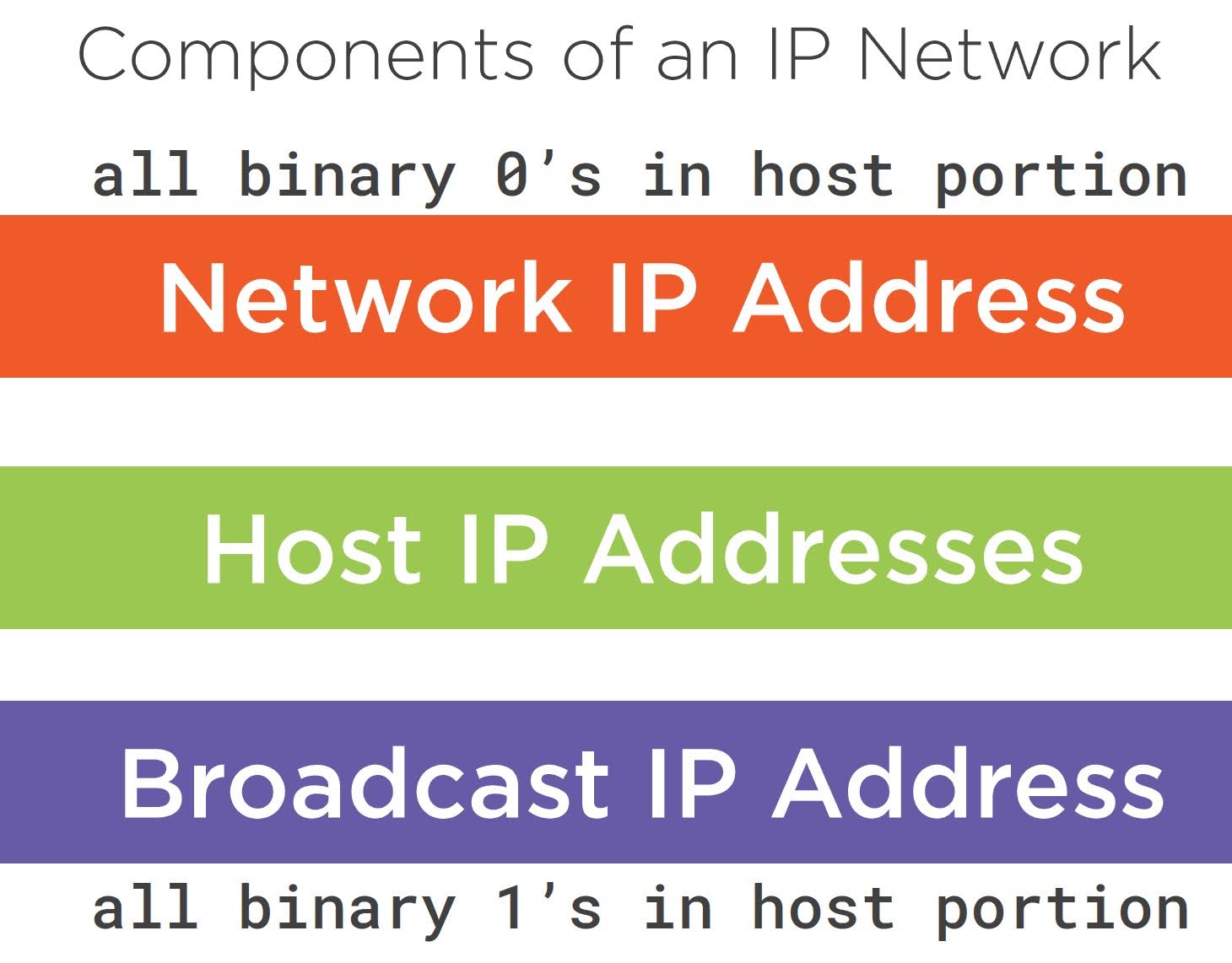
Let’s start some subnetting. Let’s take a look at 10.0.0.0/8. Now this address, this is a private IP address range. It is a network address, right? The first 8 bits, the first octet is our network portion, the last three octet are our host portion. The difficulty with this address is that with 24 bits in the host portion here, that means that we can have up to 16,777,214 unique host IP addresses within this network. Well, if you’re like me, you don’t have 16 million devices in your home, and chances are if you’re already working in IT, you should notice that there aren’t typically 16 million devices connected to one single network. Usually what happens is every area within an organization will get its own unique IP network. We don’t want to use this massive network IP space, we want a smaller one. 10.0.0.0/8 can also be represented as 10.0.0.0 with a 255.0.0.0 mask. This also is representative of a range of addresses. The range of addresses starts at 10.0.0.0, and goes through 10.255.255.255. If we convert this to binary, right, what I can do here is I can put my network address up on the top, that first binary address here, all I did there was convert 10.0.0.0 into binary. The very bottom address there is my subnet mask with 8 bits in my network portion, there’s 8 ones there, followed by 24 zeros, so that’s my subnet mask, and then in the middle, the binary address in the middle, that is my broadcast address. We know it’s a broadcast address because if we look in the host portion, we see that there are all ones in that address. What this means is that I have a range of addresses from 10.0.0.0 through 10.255.255.255, then I could manipulate to do what I need it to do. If I draw a line between my network and my host portion here, that orange line is that division between the network and the host portion, and what I can do as an engineer is I can actually manipulate where that line is in my address, right? I can change my subnet mask. Let’s take a look at how we do that. Well, what if I take a look at the address, 10.0.10.0, just as an example here. Well, 10.0.10.0, right now, that is a host address on the 10.0.0.0/8 network. I know that because there are neither all zeros, nor all ones in the host portion of my address. However, there is a section of this address that has all zeros in it, and we could move the subnet mask over, right? I could move the subnet mask from my /8 position over to a /24 position. All right, if I count the number of bits to the left side of that line, you’ll see there are 24 values there, and then there are 8 bits left in the host portion. What that means is that mask is at /24. Theoretically, here, what I could do is I could apply a /24 mask to 10.0.10.0, and still have it be a network address. That network address then, I could find out what my broadcast address is by putting all ones in my host portion, and then I could use that to determine my range of addresses in this network, 10.0.10.0 through 10.0.10.255, all right, all I did was move that mask. Now you might be asking yourself a couple questions here like, why did I move the mask, or what rules allowed me to move the mask? Well right now I’m just doing an explanation of this, showing you that with the 10.0.0.0/8 subnet, out of that, I can just change the mask a little bit here, and as long as I have a section of it that has all zeros in the host portion, I can create a new network address here. The new network address will then give me a smaller range of IP addresses to work with, making a much more manageable subnet to assign to a group of devices. 10.0.10.0/24 is a range of addresses that falls within the 10.0.0.0/8 grouping. If I take the 10.0.0.0/8 and I represent it as this big orange bar, that big orange bar is a representation of all of the addresses in the subnet, and then what I’m doing here is I’m carving out a little piece of it, that purple bar there, and that purple bar is just a small section of the entire 10.0.0.0/8 network. I’m just carving out a little piece here so that I can use in another example. If I do this a whole bunch of times, what I find out is that I can actually have a lot of network addresses within the 10.0.0.0/8 network. Here I have 10.0.0.0/24, 10.0.1.0/24, 10.0.2.0/24, and so on. These are just successive ranges of addresses using a 24‑bit mask. Additionally, I can take that 10.0.0.0/8 network, and I don’t have to use the same mask everywhere to subnet it, I can use a /24 when I find it appropriate, I can use a /22 when it’s needed, I can even use a /16 or a /30 mask, all these addresses fall within the range of 10.0.0.0/8, they just have a different mask. Also, you’ll notice that each one of these address ranges is its own unique set of addresses, so that the range of addresses, 10.0.10.0/24 doesn’t overlap with 10.0.16.0/22. Those two network address ranges are completely unique and separate. As a matter of fact, there are rules we have to follow so that our addresses do not overlap when we’re assigning them to networks and devices in our system. This system here is called Variable Length Subnet Masking, and what you’ll commonly find is that in industry when you’re looking at how networks have been deployed, you’re going to find out that most networks are deployed using Variable Length Subject Masking, and you’ll find a range of mask lengths associated with network addresses in an any given enterprise network environment.

Advanced Subnetting

Now, I went over just a brief view of what subnetting is. If you want to be good at networking, you’re going to really need to understand the depth to which subnetting occurs, alright. Network layer addressing and operation for the Cisco CCNA 200‑125 and 100‑105 exams, that article is going to do an extremely deep dive into IP addressing, it will tell you everything that you need to know about how to take any network address and break it into smaller subnets, it’ll give you some exercises that you can walk through, along with myself as I’m instructing it, and when you’re done with it, you will have such a solid understanding of IP addressing, it’ll make the rest of networking seem a lot easier to understand.

Summary

Let’s wrap up what we looked at here. We looked at some address type review, the network address, host address, broadcast address. Knowing that is the most critical component to knowing how to subnet. We looked at then how he can break a network into smaller networks. We looked at 10.0.0.0/8, and we just started moving the mask and played around with creating new subnets with a /24‑bit mask that all fall within the 10.0.0.0/8 range. Then we took a look at variable length subnet masks and saw that we can apply different lengths of subnet masks to our network addresses as long as we don’t have any overlapping addresses. Let’s move on to our next section here. We’re going to talk about IPv6 addressing.

Introduction to IPv6

Introduction

This next chapter, we’re going to talk about IPv6. Our goals this chapter will be to review the IPv4 address size and then compare it to the IPv6 address size and take a look at how IPv6 addresses are written. Additionally, we’re going to look at how we can shorten our IPv6 address to make it easier to write and say. Next, we’re going to take a look at how we can acquire IPv6 addresses on our devices, and then last, we’re going to take a look at some IPv6 tunneling.

Address Sizes

Let’s do some review of the mathematical terms that we need in order to do some IPv4 and v6 addressing. First, we have a bit. A bit is just one value, either a 1 or a 0. A nibble is 4 bits, alright, so it’s going to be something like 1010 or in hexadecimal, 1010 is A, which we write 0xA. Alright, 1010 is a decimal 10. It’s a hexadecimal A. We also have a byte, and that’s 8 bits. It’s also 2 hexadecimal values. Here, with 11001001, I’ve written the hexadecimal value C9. A hextet, then, is 16 bits long, which is 2 bytes, and that is represented by 4 hexadecimal values. That hextet is important because IPv6 addresses are written in hexadecimal, and they’re written in hexadecimal values in sets of four just like that hextet.

Let’s take a look at our IPv4 address size. Our IPv4 address size was 32 bits long, and it was broken into 4 sets of 8 bits, which we called octets, so it’s 4 octets long. Those four octets long, if we write it out in binary, represent those 32 bits, here we have 192.168.10.10 written in binary. If we take a look at IPv6, IPv6 addresses are substantially longer, as a matter of fact, they’re four times as long as an IPv4 address. And it doesn’t mean we get four times as many addresses. We get an exponential number of addresses more. Here 128 bits long is 32 nibbles or 32 sets of 4 values or 32 hexadecimal values. It can also be broken into eight hextets, and that’s exactly how we write it. The address below, 2001:0DB8:0002:008D:0000:0000:00A5:52F5. That is one big address, and it is quite hard to read. It’s quite hard to write. In IPv6 addressing, we tend to avoid these super long addresses. If we convert this to binary, you’ll see that we have a lot of values there making subnetting this a little bit challenging if we have to convert to binary all the time. I rewrote those binary numbers out there right below. That’s a lot of binary values to work with. We try to avoid the binary when working with IPv6 whenever possible. Realistically, it was actually designed this way so we don’t have to do this constant conversion to binary in order to manipulate the address like we do in IPv4. The IPv6 addresses, just like IPv4 addresses, are broken into two portions. We have a network portion of the address and then an interface identifier portion, which is just like the host portion of our address.

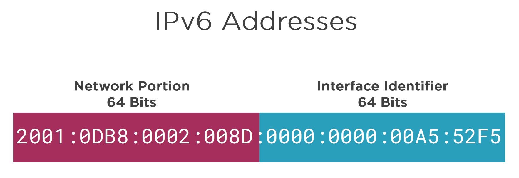
The divider for the network portion and the interface identifier portion is typically at 64 bits, when we have a network implemented with some devices on it, typically we’re going to use a /64 mask on that network so that the first 64 bits are the network portion and the last 64 bits are the host portion. We typically don’t apply much variable length subnet masking when we’re using IPv6 addressing, at least not in the standard recommended practice today. If we look at this address, we can write this address in a much shorter fashion. Alright, that’s too much address to write down and remember and say. What we can do is we can eliminate leading 0s. Now a leading 0, if we take a little sidestep here, leading 0 is something like this. If I gave you a dollar or I gave you $01 or I gave you $0001, those are all equal to a dollar. What I’m writing and saying that I can just drop the 0s that come before the 1 because they’re meaningless. That changes if I try to put the 0s after the 1. If I gave you a dollar or I gave you $10 or I gave you $1000, those are all substantially different things. I definitely would prefer the $1000 over the $1. These three values are not equal to $1. When we are working with this, we need to make sure that we can eliminate the leading 0s, but not the 0s after the value.

Here, we’re going to look at each separate hextet and eliminate leading 0s in it. We can start with 2001, 0DB8 can be shortened to DB8, 0002 can be shortened to 2, 008D can be shortened to 8D, 0000 and 0000 can be shortened to 0, and then last, 00A5 can be shortened to A5, and then 52F5 can’t be shortened because there’s no leading 0s. Once we’ve gotten rid of those leading 0s, it makes the address substantially shorter. We can make it even shorter yet, and the way we do that is that we can actually take successive hextets of 0s and replace it with a double colon. We can eliminate sets of 0s with this double colon. :0:0 here can be replaced with that double colon. Now our address becomes 2001 :DB8:2:8D::A5:52F5. That is a lot shorter to say than that address that’s written up at the top. There are some caveats to this. You have to be very careful. We can only use one double colon in an address. Typically, we place it between the network portion and the host portion to make it very easy to set up, configure, and understand how our network is set up. Some errors we can make. This is a correctly formatted address. If we look at this one, it has two double colons in it between the 8D and the A5 and then the A5 and the 52F5. We can’t do that because we won’t know where all the 0s go. For this example here, if we take a look at what happens with that when we have two double colons, we don’t know where the 0s go. This could be 2001 :DB8:8D:0:A5:0:0. It could be 2001 :DB8:8D:0:0:A5:0. It could be either one of these, so we don’t know. We can only use one double colon in an address. This last one here, 2001 :DB8:2:8D:A5:52F5. We have no double colon in there at all, we have no idea where the extra 0s go, this won’t be recognized as a valid address because there’s not enough bits in it.

How Many IPv6 Addresses?

How many IPv6 addresses do we have available to us? It’s hard to fathom this. In the interface identifier portion alone, alright? Just in our host portion of our address, we have 2 to the 64 possible addresses. This is about 18 billion billion addresses, right? This is an enormous number. That number right there, just the number of host addresses on one IPv6 network is 18 billion billion. That means that if we took every star in the Milky Way galaxy for that one IPv6 network, we could give each star in the Milky Way galaxy 184 million IP addresses. That’s impressive, right? We could give every insect on earth would receive two IPv6 addresses. Each bug on earth gets two IPv6 addresses. We could even do this with grains of sand, right? There’s about as many grains of sand on the earth as there are insects, apparently. I don’t know who goes around counting this stuff, but anyway, there are about two IPv6 addresses for every grain of sand for one single IPv6 network. How many IPv6 networks are there? There are 18 billion billion IPv6 networks. We just have this unbelievable number of IPv6 networks available to use along with host addresses.

Demo: Examine IPv6 Information on a PC

Let’s do a demonstration here and take a look at the IPv6 information on our PC. We can also examine dual stack on a PC, meaning that we’re going to have both IPv4 and IPv6 running. I’m on my Windows 10 workstation here, and what I want to do now is go into the network configuration for my network interface card. To do that, in the lower right-hand corner of my screen in the system tray here, there is usually a little computer with what looks like a little pitchfork next to it, which is actually the Ethernet cable and the end on it. If I right‑click on that and do Open Network and Sharing Center, that will bring me to a screen here where I can go into change adapter settings, and then I can right‑click on my Ethernet connection and go to Properties. In here, this before is where we set our IP version 4 address, and if we scroll down a little bit here, we can also set IP version 6. Right now I have that box unchecked, which is something I like to do on my work stations. IPv6 on Windows machines tends to get automatically configured. On Windows machines, there’s a preference to use IPv6 to communicate on the Internet over IPv4, I try to turn that off to make sure that I’m only using IPv4, and that tends to make communication a little bit speedier. I turn it on only when I’m working with IPv6. We’ll check that box and we’ll click Properties. What will happen here is it’ll give me the window now to manually configure an IPv6 address. As soon as I’m done with this demonstration, we’re going to look at other ways that we can obtain an IPv6 address on our workstation. Mainly this automatic version up on top here. For the time being, we are going to do this manually. The address I want to put in here is 2001db8, and then I’ll put 10, double colon 10. Now 2001db8, that is a documentation IPv6 address, it is not a public address. There is no private addressing in IPv6. We’re just going to use that address as our documentation address, which is not routable on the Internet. I don’t have a router connected to my system, I’m going to leave the default gateway blank. I do have another IPv6 workstation connected to the switch that this workstation is connected to. If I open up command prompt now and I do an ipconfig, it should show me both my IPv4 and my IPv6 address. Here is my IPv6 address, the 2001:db8:10, double colon 10, and then my IPv4 address here 192.168.11.10. What this is called now is dual stack. It means that I have both IPv4 and IPv6 running on my workstation now, and I can use either the v4 or the v6 address for communication now. I can demonstrate this by trying to ping 192.168.10.100, which is the IPv4 address of my other workstation. I can also send a ping message to 2001:db8:10 double colon 100, which is the IPv6 address of the same workstation. Now I can send messages back and forth between our workstations in both IPv4 and IPv6. If I issue ipconfig again, what we’ll notice here is that my IPv6 address actually has two of them shown here. Now this is something unique to IPv6 is that every single interface in IPv6, if it’s going to talk on a routed network, will require at least two IPv6 addresses. This is unique to IPv6. We don’t do this in IPv4. This first address, this is called our unicast address. Typically, that’s the global unicast address. The address right below it, the one that starts fe80, this fe80 address is the link local address and that address exists only within the layer two network and never, ever, ever leaves it. The way I look at this address is it’s kind of like a MAC address that we’re going to use up at the network layer. All right, it’s a unique identifier in IPv6 for this specific workstation. But that address will never, ever, ever leave the local Ethernet network, which is exactly how MAC addresses work. MAC addresses exist on a layer two network and they’re never routed off of that network. This link local address is used to make IPv6 work. It’s automatically configured, for the most part, we can leave it be. The one that’s most important to us is the global unicast address. That address is going to allow us to communicate out to the Internet using IPv6. Let’s go on and take a look at how else we can acquire IPv6 addresses on our workstation.

IPv6 Address Acquisition

Now that we’ve seen IPv6 on our work stations, let’s take a look at how we acquire IPv6 addresses. The most common method here is called SLAAC, which is stateless address auto configuration. By default, when we connect a device to a recently configured network, in this case, I just have a PC connected up to a router, a layer‑3 device. What will happen is if that router has an IPv6 address configured, the router is going to send out this advertisement saying, hey, I’m a router and I’m on this network. The PC will get that advertisement. It will then say, oh, I’m on network 2001:DB8:4A. The PC can then pick its own IP address. Windows machines are going to pick their own 64‑bit random interface identifier value, and add it on to the network portion of the address. Alright? Here, 2001:DB8:4:A and then a random value gets attached to that number, and then that becomes the Windows IPv6 address using SLAAC. On UNIX, Linux, Mac machines or anything that’s running a more standard version of UNIX code, those are going to use something called a modified EUI‑64 format for the address. What they’re going to do is they’re going to take the Mac address, which is 48 bits long, and they’re going to modify it just a little bit to make it 64 bits long. The way we do that is we break the Mac address in half, and then in the middle, we put FF:FE in the middle of our Mac address. That then becomes the beginning of our host portion or our interface identifier portion for our address. We have to do one more thing yet, and that’s take the first eight bits, and what we’re going to do is we’re going to take that seventh value of our binary and whatever value it is initially, we’re going to flip it so that it’s the other one. Here the first two values are 00 from a Mac address. What I do is I take 00, convert it to binary. I flip the seventh bit from a 0 to a 1, and then I reconvert it to hexidecimal. My new address here starts with 02 instead of 00. This address then becomes the interface identifier portion for my IPv6 address. Once I’ve decided what that address is, then I send a message back to the router saying, hey, I’m a neighbor now and here’s my address. The router will then record that address in a table so that it knows which IPv6 address at layer 3 is associated with which Mac address at layer 2.

IPv6 DHCP

A second way we can acquire IPv6 addresses is we can actually use an IPv6 DHCP server. This DHCP server, what it’ll do is when we put a device on the network, the workstation will send out a message saying, hey, I need an address. The DHCP server will then respond with an IPv6 address. This works very similarly to how it does in IPv4. We’ll spend some time doing a deeper dive on IPv4 DHCP in the last chapter of this article. Tunneling IPv6. Now IPv6 is not incredibly prolific across the world yet. The internet backbone itself is full of IPv6; however, oftentimes, users at the end in an enterprise organization or in a home network don’t actually have access to an IPv6 internet. In order to do that, what I’ve drawn here is I have Hurricane Electric. He.net is over on the left‑hand side of the drawing. That’s my IPv6 internet. Hurricane Electric has a pretty massive deployment of IPv6 and has a pretty easy setup for you as an end user to be able to access the IPv6 internet. That will allow you then to build a tunnel to Hurricane Electric to get you IPv6 internet access. The way that works is here I have a workstation over here on the right‑hand side of the screen. That’s an IPv4. What I do is I have this connection with a router, and what I can do is I can actually build a tunnel through the IPv4 internet, which my PC is connected to, to the IPv6 internet, and that allows me to get access to it. The way that tunnel works is I take IPv6 packets, and I put them inside of an IPv4 packet and then I send that across the internet. When it gets to the IPv6 network, I take the IPv6 packet out of the IPv4 packet, and now my traffic is over at Hurricane Electric where it can freely roam the IPv6 internet and then get back to me across that IPv4 tunnel across the internet. Now our IPv6 internet over there, we are now connected to it with that tunnel. From the perspective of our workstation, it may look like there isn’t even actually an IPv4 internet available at all because we’re just doing that specialized tunnel. Microsoft will oftentimes automatically build a tunnel for you over to Microsoft and give you an IPv6 address as well.

Summary

To wrap up what we’ve done here, we looked at the IPv4 address size, and then we took a look at IPv6 addresses, saw how much larger they were, and then looked at how we could shorten that address to make it easier to write and say. We looked at how IPv6 addresses are acquired; we can either manually configure them like we saw in the demonstration, we can use Slack, or we can use an IPv6 DHCP server. We’ve wrapped up this chapter by taking a look at how we can tunnel IPv6 traffic through an IPv4 network, giving an otherwise island of IPv4 networking access to IPv4 internet. I hope you’ve learned something from all this IPv6 information, know that IPv6 is not incredibly prolific on the Internet yet, enterprise organizations around the world will most likely not be in a rush to implement IPv6 unless they absolutely have to, there’s just not a lot of cost benefit to it.

Ethernet and Switching

Introduction

This next chapter is Ethernet and Ethernet Switching. Now Ethernet is prolific in nearly every single network that you are going to see in your career, and Ethernet switches, you’re also going to be working with constantly. Our goals this chapter is to introduce Ethernet and first talk about the foundations of Ethernet, which use these six letters to describe it, which is CSMA/CD. We’ll look at how that operates, and give us a good introduction into Ethernet. Once we understand what CSMA/CD is, we’re going to take a look at collision domains. Now collision domains aren’t a big part of modern networks, but it really establishes the history of how Ethernet actually works. We’re going to take a look at what that is. Next, we’ll look at the duplex and speed options of Ethernet. We’ll take a look at the Ethernet frame, which is the mechanism used to actually move data across a data network using Ethernet. Last, we’re going to take a look at a switch and see how switches operate, and actually do a demonstration where we log into a switch, that’s a managed switch, and take a look at that MAC address table.

Ethernet

Before we get into talking about Ethernet, I always think it’s important to come back to the OSI model here. For this topic, we’re exclusively focusing on layer two, the data link layer. Any time we’re discussing Ethernet, or frames, or switches, we’re talking about layer two, the data link layer. The data link layer is responsible for protocols that allow traffic to move in between devices that are locally connected together, so devices that are all hooked up to the same device. When we talked about this during the OSI model chapter, we saw that Ethernet is used almost everywhere. We use it a lot on the Internet, it’s used in our home network, it’s used in our home network to connect typically to our cable modem or our DSL modem, and then it’s used in the data centers where we are connecting to servers to download websites like xxx.com. Ethernet, like I said earlier, is incredibly prolific in data networking. As a matter of fact, most likely, you have a device like this sitting some place in your home that allows you to connect to your internet service provider and provide wireless internet access in your home, as well as wired internet access, and we’re doing this by using Ethernet, actually two distinct and unique types of Ethernet, one is wireless Ethernet and the other is wired Ethernet. Wired Ethernet, if you look on the back of that device that’s sitting in your house, you’ll see some ports like this like these yellow ones on this wireless router, right? We plug our internet connection into one of these ports, and then we have four or five ports, typically, that allow us to connect devices to them. These ports that we’re looking at here, this is Ethernet and these are Ethernet switches that are built into this device. If we go into an enterprise network, you might see a switch like this. This is a Cisco Catalyst 3750g switch. This is nothing more than a very large version of the one that you have in your home. It has a lot of extra features on it that we could enable, and we’ll talk about some of those, but understand that effectively, this device is almost identical to the device that you have in your house, it’s just much larger and much more expensive. If we look at this in a data networking closet, here this networking closet has some Hewlett Packards, some HP switches that are installed, and this might be a closet that you walk into in an enterprise business. This could easily be just a data network closet where all the computers in a area of a company all connect to one closet here through this patch panel and then connect down to that switch. For now, understand that switches are typically used to connect all the devices in our network together.

Carrier Sense Multiple Access with Collision Detection

CSMA/CD. These six letters are what the original designers of Ethernet used to describe its operation. Now CSMA/CD stands for carrier‑sense multiple access with collision detection. Let’s take a look at this example here. What I have is, I have seven computers all hooked up to one cable, all right. And this is an old style of networking called a bus network. And what we used to do is, you would have these computers. In fact, I worked in an office, when I was a structural engineer, I worked in an office and supported a network just like this. Each one of our drafters who were drafting homes for customers, they were creating the plans on these computers. They were all connected together with this one single wire. It looked kind of like a wire that you would use to connect your cable TV to. And there were these little T taps that would allow me to break the one long continuous wire and then hook up each PC to this network. This is how the initial version of Ethernet worked. All the devices were hooked up to one single cable. Now Ethernet doesn’t work this way today. At least we don’t configure it this way today. But we’re still using CSMA/CD. Let’s take a look at how that works. The idea here is that when a device, let’s say the maroon device in the lower left‑hand corner, wants to send a message to any one of the devices on this network. What that device would do is, it would send a pulse of electricity. It would either have a + or ‑5 volts or no voltage on the wire. And what that does is, that on off of the 5 volts and no 5 volts, that creates a signal that allows us to transfer a message. It creates this pulse of 1s and 0s, ons and offs. And what happens when we do that is, when the maroon device communicates on this network, all the devices on the network hear the messages. Only the intended device that the maroon device is trying to talk to will typically respond, but all the devices on this network can hear the conversation. If now the green device wants to talk, the green device can talk as well here. And what’s going to happen is this. The multiple access here means that all these devices are sharing the same wire, much like if you had a landline in your home, and that landline in your home had multiple extensions to that phone. That maybe your sister was talking on the phone, and you picked up the phone and you could hear your sister talking. You wouldn’t get a dial tone; you’d get your sister talking. This is the same thing. If the green device is talking and the maroon device wants to send some information on the wire, well, the maroon device will listen to the wire and say, oh, there’s somebody talking on this wire. I can’t send any data. the maroon device has to wait until the green device is done. However, it’s very easy to have an accident where both devices listen to the wire and hear that no devices are currently communicating, and then the green device and the maroon device here both start communicating at the exact same moment. What’ll happen here is, they’ll both send a 5‑volt signal onto the wire. When both devices send a 5‑volt signal onto a wire, what that does is, it creates a 10‑volt signal. All of the devices on the network are designed to recognize signals that are beyond 5 volts. When that happens, when they get this surge of voltage on the wire, a collision occurs. And that means that two devices, two or more devices, tried to communicate at the same moment. The network said, yep, you can’t do that. We’re going to stop the conversation. We’re going to back off and wait a random period of time and then start to listen to the wire again to see if it’s ready for me to send data. Carrier‑sense, we’re going to listen to the wire, multiple access, there’s numerous devices accessing the same wire, and then collision detection. What we’re doing there is, we’re saying if we hear a signal that is greater than 5 volts, like 10 volts, in this case, we’re going to create a collision. We’re going to tell all the devices to stop listening, discard anything they’ve just received, and wait and start over again. A collision domain now is a group of network devices that will simultaneously detect a voltage spike. And that voltage spike, remember, is just multiple devices sending data at the same time.

Duplex and Speed

Let’s take a look at duplex and speed, Duplex and speed here. The duplex of a connection in Ethernet can either be half or full. This animation on the left‑hand side of the screen here, between the blue and maroon computers, this is representing half duplex communication.

It means that one device communicates at a time. The blue device can send information to the purple device. The purple device can send data to the blue device, but we cannot send data simultaneously. This is very similar to how a walkie talkie would work in real life, right. If I want to talk to my buddy on the walkie talkie, I hold the button down, that allows my communication to be sent to anybody listening at that moment. But what I can’t do when I’m talking is listen to other people talking on that device, right? I can either talk on it or I can listen on it, but I can’t talk and listen at the same time. Which brings us to full duplex communication. Full duplex communication means that two devices can communicate at the same exact time.

Here this is more like a telephone conversation. When I pick up my cell phone and I talked to my mother. I can hear my mother talking through the ear piece and I can talk to her at the same time she’s talking through the microphone. That is full duplex communication. When we have networks with full duplex communication, when we have Ethernet networks using full duplex, collisions are not possible. All right, because both devices can send data onto the wire at the same time here. When we’re using full duplex, typically we don’t have to worry about collisions at all. In a modern collision domain, if we take a look at this, modern collision domain is really just going to be a half-duplex connection between a PC and a switch. All right, and that that half duplex connection is the case where we can have a collision domain. Why would we have this set to half duplex? Well, it could be many reasons. One of the reasons is that it could be an old device. Another reason is that it could be an old switch or old wiring. Or maybe we’re just doing some experimentation and we force the connection to be half duplex. That half duplex configuration here makes it so that the switch can’t send information to the PC and the PC can’t send information to the switch at the same time, they have to take their turns. That causes a collision. Most modern networks are full duplex, meaning that the PC can send to the switch and the switch can send to the PC, both simultaneously. Right, and most network connections that you use in modern networks are going to be like this. We won’t even have a collision domain to worry about. The speed of Ethernet here, we have a 10 Mb Ethernet. That’s the original Ethernet speed from 1982. Later on, we get 100 Mb Ethernet. We have gigabit Ethernet now, which is a very common speed of Ethernet in modern networks. Ten gigabit Ethernet, you’ll see 10 Gb Ethernet used to connect different ISPs together, as well as 40 Gb Ethernet. There’s even 100 Gb Ethernet now. Most of these higher speed Ethernet connections, they’re used in data centers and in the connections, in the wide area network connections, that allow ISPs to communicate with each other. We’re going to see these super high speed Ethernet connections when we are aggregating a bunch of traffic in between Internet service providers. We’re going to see the slower speeds, gigabit and less, inside of our networks that we use on a daily basis. The bottom three here, gigabit, 10 Gb, and 40 Gb all require full duplex. CSMA/CD doesn’t really even apply to the 1 Gb, 10 Gb, 40 Gb, 100 Gb, and further Ethernet connection speeds.

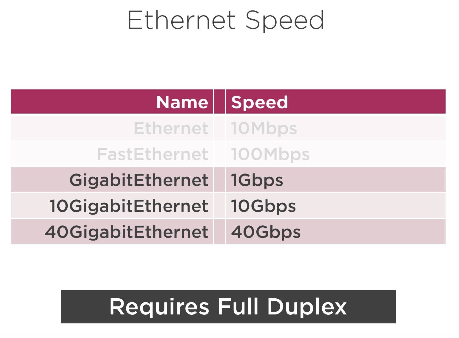
Ethernet II Frame

Ethernet uses a frame. Ethernet II is the protocol name, actually, and Ethernet II frame, it’s the same frame we’ve been using since the early eighties for Ethernet. Although Ethernet’s protocols have changed, the speeds of the links have changed, duplexes have changed, what hasn’t changed actually is this frame. And what we do with the frame is the frame is the mechanism that we use to move data across an Ethernet network from one device to another. This frame is composed of several different pieces here. In the middle of the frame or actually in this picture, it’s off to the far right, is our data, alright? And our data is either going to be some layer‑2 information that we’re transferring, or it’s going to be some layer‑3 information. If it’s layer‑3 information that we’re transferring, that should be a packet, most likely an IP packet using IP addresses at the network layer. We don’t have to transfer IP data. There’s some other data that we can transfer with frames, but just know that that data, that gray area. is the data that we’re actually transferring here. The rest of the information in the blue highlights is the frame information, and that’s what Ethernet is going to use to actually move the data. Here this frame is nothing more than a chunk of data, the packet information or other information in the gray, combined with a data link layer header.

In this case, it’s an Ethernet header, and that Ethernet header has several components here. In this case, everything in the blue highlight here, Destination MAC Address, Source MAC Address, Type, and FCS, these are all part of the Ethernet header. Alright?

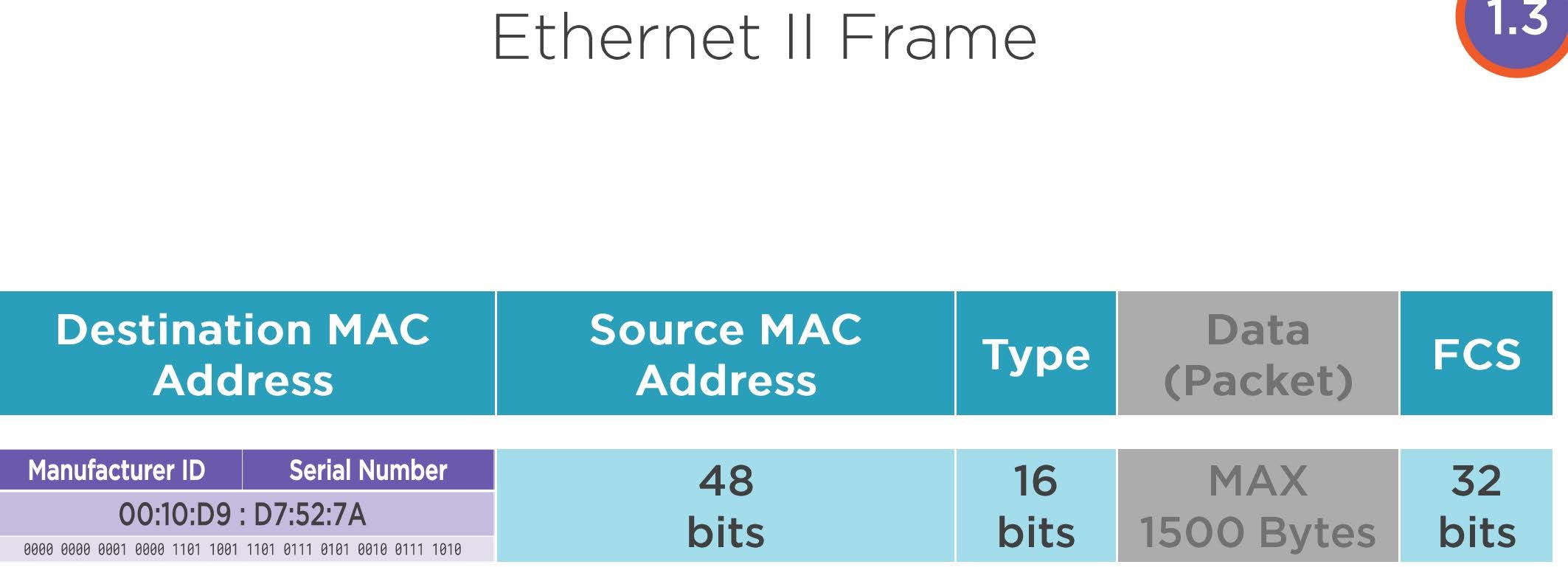
This is the data link layer header or the Ethernet header. The data here, that’s our payload in the gray. Let’s look at each field here. The destination MAC address, alright? The destination MAC address and the source. MAC address, these are layer‑2 addresses or layer‑2 identifiers that are specifically tied to a network interface card. Now a network interface card is the device that we actually plug in our Ethernet cable into. Alright? And that MAC address is composed of two pieces here, a manufacturer ID and a serial number. The first 24 bits of that address or the manufacturer ID, the last 24 bits are a serial number. These MAC addresses are configured at the factory itself. These MAC addresses are actually burned onto the network interface cards long before you receive the device. This MAC address is a hardware address that is assigned to devices right at the factory, and this is our layer‑2 address.

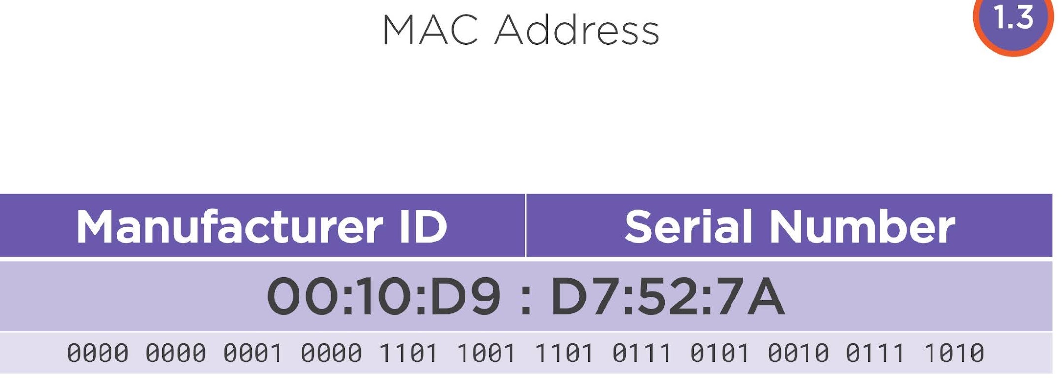
We have both a source address and a destination address for our Ethernet frame. The next field here is that Type field. The Type field is going to tell us what type of data is being transferred. Is it layer‑3 data? Is it some other data that we’re transferring? The Type field will indicate what that is. And then the last field here is the Frame Check Sequence, the FCS. That does something called a cyclical redundancy check. And effectively, what it does is it takes all the information in the frame, it runs it through a little algorithm, and computes a value. That value is put into that 32‑bit field at the end of our frame called the FCS. Then when the frame is received by the other device, the other device does the same calculation again and checks to see that the FCS of the received frame is exactly the same as the FCS of the sent frame. There is a maximum amount of data that we can transfer here. It’s called the MTU in a frame, or the maximum transmission unit. The maximum transmission unit for Ethernet is 1500 bytes. Another piece of terminology that we need to use here is called the protocol data unit. Now, the protocol data unit is going to vary from layer to layer of the OSI model, but the protocol data unit here, or the PDU, is going to be the entire frame and the data that we’re transferring. Alright, our layer‑2 PDU here contains the entire frame, the source and destination MAC address, the Type field, the FCS, and the data itself.

Network Topologies

Now that we have some understanding of this frame, that there’s a source and destination MAC address in there, we have some basic understanding of the speed and duplex, let’s take a look at topologies and how we currently deploy Ethernet in modern networks. There are really, generally speaking, three types of topologies that we will see in networks. One of them I had mentioned earlier, and that’s the bus. The bus topology is just a single wire, and we tap into that single wire and run our devices off of that.

You’ll very rarely see a bus network in modern data networks. Bus networks, you would see a lot of these in the early to mid even late 90s, but they went away after the 90s quite quickly in favor of star topologies, which we’ll get into in just a moment. Ring is the second type of topology that we can use here. Ring topologies are also antiquated.

In the mid 80s to late 90s, there was a somewhat popular network topology called token ring, which was a competitor to Ethernet. And token ring used a ring topology instead of a star topology or bus. Now we don’t see many ring topologies is anymore either. They have mostly gone the way of star topologies, which is what modern Ethernet uses right now. Modern Ethernet is really prolific. It won the battle against token ring in the 90s, and really, we’ve moved to the star topology for almost everything. The bus topology, like I said, we’ve taken a look at this before when we looked at CSMA/CD. Means that if a device sends a message, all the other devices can receive that message. If we look at bus topologies connecting types, the picture on the right here, that’s what I was talking about earlier when I supported that network at that architecture company with supporting the drafters. What we used there was these connectors. They’re called little BNC connectors with some 10BASE2 cabling. The picture on the left, that is some older Ethernet. That’s using the 10BASE5 wiring and vampire taps. They actually of these taps that you have to drill into that yellow cable and install these taps to get all this to connect together. That’s the original Ethernet on the left. Next generation Ethernet is on the right, and we use neither of these any more in bus topologies. All right, ring topology. What we would do is, we’d have this little token that would spin around a ring and then, as devices needed to transfer data, they would attach messages to this token. And then, as a device would receive the token with a message for it, it would take the message off the token, put it back on the wire, and the process would start over again. This was a very efficient way to send data. The problem was that IBM made it extremely expensive to implement it, so it just never took off, not in the way that Ethernet did. This device here, this is called an IBM token ring MAU, or Media Access Unit. And this device, what it did was, it hooked up all of your computers to this one device, and then it would pass the token around that network. The star topology is really what is popular. This is what we see everywhere.

Now, this device that I have drawn in here, this box with a double‑headed arrow in it, that’s called a hub. That is a Layer 1 device. We’ll talk about hub operation a little bit later on. Hubs we don’t see very much in networks, but the star topology originally came from using this hub. Now a hub is nothing more than a multiport repeater. I put a signal into it and then all the other devices on that network hear it. In this case, if the green device sent a message, every single device on this hub would hear that message. And if the green device and the purple device sent messages at the same exact moment, there would be a collision. Switching takes care of that. We’ll take a look at that in just a second here. Here is a picture of a Cisco Catalyst switch. If this were a hub, it would look almost identical. We would just change the name from switch to hub. Let’s talk then about this Layer 2 switch. All right, this Layer 2 switch, what’s happening here is, if we were to use that as a hub, like I said, when two devices sent messages at the same time, there would be a collision. Ethernet switching allows us to prevent collisions. All right, switches break up collision domains. Let’s take a look at how this switch works. Switches keep track of MAC addresses. What switches will do is, they’ll actually read the frame headers. They read the frame headers, and they see what source MAC address is being received by a port. What’ll happen then is, the switch will then keep track of all the MAC addresses assigned to each device that’s connected to the port. What I’m going to do here is just use two numbers for a MAC address, two hexadecimal values which look like a representation of a number and a letter. What will happen is, as these devices send data into the switch, a little chip on there is going to read the source MAC address. In this case, A7 is going to put its source MAC address in the frame header, and then it will populate this MAC address table. Now if I want to send a message to device 6E, the switch knows that that’s connected on port 1. All right, now if we have this message, let’s say that A7 wants to send a message to device B3. Well, what’ll happen now is, A7 will create a frame, the source MAC address of the frame will be A7, the destination MAC address of the frame will be B3, which I’ve shown in that little envelope. When the switch receives that message, it’s going to look at the destination MAC address and compare it to the MAC address table. Here if we have B3, it’s going to look in the MAC address table, that is going to port 2. Now we can create a little virtual circuit inside of the switch and send a message between A7 and B3, and none of the other devices on our switch hear that conversation. We can have this continuous message happening between A7 and B3, and none of the other devices will hear it. Then if the device on the bottom in the green sends a message from device C2 to device 6E, we can see the same process happening. While A7 and B3 are talking, this message destined for 6E, we can look that up in the table, see that it’s destined for port 1, and then send our message along the way on its own little virtual circuit. Now we can have both C2 and 6E talking at the same time as A7 and B3. No collisions occur here because we create these little virtual circuits inside of the switch that only allow communication between the source and destination MAC address of the frame. This is really effectively what the switch is doing for us. Broadcast messages. Now broadcast messages are super important in Ethernet, all right. Ethernet is considered to be a broadcast network type, and what happens here is, if we put all Fs in the destination MAC address field, that is called a Layer 2 broadcast address. Now we talked about Layer 3 broadcast addresses, and those are completely different. Layer 3 broadcast addresses are rarely used, versus Layer 2 broadcast addresses, which are constantly used in Ethernet. A broadcast message in Ethernet is when the destination MAC address of the frame is all Fs. What this means is that the frame is going to be sent out all active interfaces except the interface that received it. Let’s look at this in operation. Let’s say that A7 needs to send out a broadcast message, it creates a frame with a destination MAC address of all Fs. I’m just using two Fs here to represent all Fs in the destination MAC address field. When I send that to the switch, the switch will read that destination MAC address. It won’t even consult the MAC address table. What’s going to happen is, it will recreate that frame and send it to all the devices on the network. A broadcast domain then is a group of network devices which will all receive a Layer 2 broadcast message.

Demo: Examine the MAC Address Table

Let’s do a demonstration now, where we examine the MAC address table of a switch. What I have set up here is the switch with six devices connected to it. The switch is represented by that gray rectangle in the middle, with arrows pointing in the opposite direction. What the switch actually looks like is this right here. It’s a Cisco 2960 switch. You can pick these up on eBay for $30 to $50, and what I’ve done is I’ve just connected several PCs to this switch. The PC that we’re going to be looking at is the blue PC over on the far left‑hand side of the drawing. And I’ve listed the MAC address for that PC on there. The other PC that I have access to that we can ping, it’s connected to port 3, it’s the black PC there. Effectively what I’ve done here is I’ve taken the two PC’s that I used from the IP addressing demonstration and I’ve implemented them here. Let’s connect to that blue computer now and take a look at the MAC address of that PC, as well as the MAC address table of that switch we’re connected to. Here’s my windows PC. I’m going to open up command prompt. In the previous demonstrations, we’ve looked at the ipconfig command, which shows us our IP address and subnet mask, it’s telling us our layer three addressing information. If I issue another command here by just adding the slash a‑l‑l to the end of the ipconfig command, what that’ll do is it’ll tell me more information about my network adapter or Ethernet card. My layer three addressing information is still listed here, but in addition to that, I also have the physical address listed here. And this is our layer two address, our data link layer address. This is also called the MAC address or the hardware address. Hardware address, physical address, MAC address, they’re all the same thing. Here this MAC address is what the switch is going to be looking at and recording in the MAC address table. In order to get the MAC addresses to populate in the table, I need to send a message to the other device 192.168.10.100. That will send a frame along with that ping message over to the other device. If I open up PuTTY, now PuTTY is an application that’s going to let me connect to my switch. All right, I have a cable connected to the switch and I can get a command prompt with the switch then. If I issue the command show mac address‑table, now, dynamic, it’s going to show me the MAC addresses directly connected to this switch. And sure enough, connected to port 3 is the MAC address ending in 0572, which is the MAC address of my other workstation, connected to port 6 here is the MAC address of my workstation ending in 70a5. I can pull up my command prompt here again quickly and scroll down, and we can see that my MAC address is 70a5, and the MAC address table is saying that it’s plugged into port 6 of the switch. The other MAC addresses on this switch are connected to it, and we can see the ports that they’re connected to. Over time these MAC addresses will eventually age out of this table, which means they’ll just drop off the table if the switch doesn’t hear any frames from the device that’s connected to it. At the time that the switch receives a frame from the device connected to that port, it’ll re‑add the MAC address to the table. It does this so that you can move switch ports around and not have the switch fail in operation.

Summary

To wrap up what we’ve done here, we looked at CSMA/CD, carrier sense multiple access with collision detect, which is how the original version of Ethernet worked. We took a look at what collision domains were, and identified them as a group of devices that can all detect a voltage spike at the same time. We looked at the speed and duplex settings that we can apply to Ethernet. We looked at an Ethernet frame and saw the source and destination MAC addresses in that frame. And then we took a look at the MAC address table of a switch. Now we’re covering layer‑2 switching here at a relatively high level. Let’s move on to the next one where we’re going to talk about slightly more advanced Ethernet topics.

Switching Features

Introduction

In this next chapter, we’re going to take a look at switching features, which is an advanced section of learning how switches work. And our goals this chapter, we’re going to take a look at broadcast storms and how we can prevent them. We’re going to look at VLANs, which are virtual LANs that are combined on one switch. We’re going to take a look at what mirroring switch ports are. And last, we’re going to take a look at Power over Ethernet and see what value that provides us.

Connecting Switches

First of all, let’s take a look at connecting multiple switches together. With switches, we can take more than one switch and connect them together to increase the size of our broadcast domain. Let’s take a quick review of what a broadcast domain is by looking at how broadcast messages behave on a switch. Remember, this is a layer 2 broadcast because we’re talking about a layer 2 switch. That rectangle in my drawing there, with the arrows pointing in opposite directions, that is a layer 2 switch we are looking at. When a switch receives a broadcast message, it forwards that message to all other switch ports that are currently active. Well, when there are only two devices on our network, the broadcast messages only go between the two devices. When we add more devices on the network, remember that broadcast message gets sent out all the interfaces that are active. Any broadcast messages that get sent, all other devices on this network hear about it. Well, what if we connect two switches together? Now the blue PC in the upper left‑hand corner is going to send out broadcast messages. When those broadcast messages reach the top switch, the top switch forwards those layer 2 broadcast messages with all F’s in the destination MAC‑address field, forwards out all active interfaces. Then, because there is another switch connected to the top switch, when that bottom switch receives that same broadcast message, it’s going to do the same behavior. It’s going to look at the destination MAC‑address and then forward that frame out all the active interfaces, except for the one that the frame was received upon. Well, this isn’t such a bad thing, right? If we have two machines sending broadcast messages at the same time, all the machines on the network are going to hear about it, right, even if a machine on the bottom sends the broadcast message. This can get a little messy, right, over time, but the reality here is that this is how the system was designed to work. Broadcast messages get propagated out all active switch ports. Well, now, let’s imagine a case where maybe you are having a gaming party. You’re having a LAN party, and you invite all of your friends over, and you go over to Best Buy and you buy 2 Gb Ethernet switches. The 2 Gb Ethernet switches then you connect together with 2 cables, hoping that you’ll have 2 Gb connecting the 2 switches together through the 2 cables and that the people on the top switch will have much faster communication to the people on the bottom switch had there only been one connection instead. We’re trying to improve our performance here. However, this causes a pretty substantial problem in our network. All right, these two switches that we have connected together, remember, when the switch receives a broadcast message with all F’s in the destination field of the frame header, what will happen is the switch will forward those messages out all active switch ports. Now, when the bottom switch receives these broadcast messages on two switch ports, the bottom switch is going to actually send out a broadcast message out all active switch ports, including the two switch ports that connect to the other switch. Now we have two broadcast messages that got stuck in between our two switches here. Over time, as the machines start sending out more and more and more and more broadcast messages, this connection, these connections in between the two switches will be filled up with broadcast messages that have nowhere else to go. They just keeps circling in this loop in our network. All right, and that loop can just make things terrible, and it’ll actually crash the network. It’s going to cause something called a broadcast storm. All right, and that broadcast storm means that there is just too much traffic in between the two switches, there’s too much traffic that the switches are processing, which means that for your gaming network here, everybody is going to not be able to communicate with anybody because there’s just too much broadcast traffic on this network. How do we solve this problem? This broadcast storm problem we solve with Radia Perlman, who invented Spanning‑Tree Protocol back in the late ’80s. What Spanning‑Tree Protocol does is on enterprise class switches, meaning switches that you probably aren’t buying at Best Buy, on these enterprise class switches that you would use in a bigger business, what happens is when you connect the two switches together like this, the two switches go through and figure out which ports are redundant, and they shut one of them down so that now we can only use one connection in between these two switches. If you buy the switches at a Best Buy or Amazon and they’re lower end home switches, typically Spanning‑Tree Protocol is not enabled on those switches. They do not expect you to be connecting them together like this. In an enterprise, oftentimes you have to connect many switches together in an area to get enough ports to provide the users with a network connection. Here, in order to solve the problem and prevent the switches from just stopping operation in case somebody accidentally connects two of them together, we have to use this Spanning‑Tree Protocol, or STP, to shut down the redundancy and prevent these loops from occurring. And even if we have a bigger network, right, the bigger network we have here, if we have three switches all connected together in a loop, what will happen is spanning tree is going to figure out which port to shut down, shut that port down, and then prevent the loop from existing.

Intro to VLANS

Let’s move into VLANS. Let’s introduce what VLANS are. A LAN is a local area network, right? It’s a group of devices typically connected together with an Ethernet switch. VLANS really take that concept to a new level here. We have this broadcast domain that we just talked about, right? The broadcast domain is the set of devices that can receive a message with all F’s in the destination MAC address field. Here we have the device on the far left sending out a broadcast message, and all the devices are receiving that message. If I take this one switch and I split it into two switches, alright, I have two separate systems here, what I can do is create two separate broadcast domains, alright? If we look at the broadcast domain on the left, we’ll see that it has some layer 3 addressing assigned to it, and all the IP addresses on the broadcast domain on the left are in the 10.0.0.0/24 network. On the right-hand side, if we look, those also have layer 3 addresses assigned to them. Those are on the 172.16.0.0/24 network. Each broadcast domain here receives its own unique layer 3 network, and this is exactly how the technology is designed. Each broadcast domain represents one single layer 3 network. Alright, when we’re setting these up, we design our networks so that they are also broadcast domains. Here we have two unique broadcast domains connected to two different switches. Well, let me call the broadcast domain on the left VLAN 1, and I’m going to call the broadcast domain on the right VLAN 2. What I can do now is I can actually combine these two switches together into one physical switch, alright? This physical switch can be the 2960 switch like I’ve been using in all of my demonstrations. This 2960 switch actually has the capabilities to support more than one VLAN, or more than one broadcast domain. Well, these VLANS now exhibit the same properties that it did when we had them connected to two different switches. That if I send a broadcast message out from a device in VLAN 1, it only goes to other devices in VLAN 1, and if I send the broadcast message out in VLAN 2, it only goes out to the devices in VLAN 2. The way that this is configured is that each one of the switchports has a number assigned to it, right, we have FastEthernet 0/1 for a port, FastEthernet 0/2, and what we do is we just configure each switchport through a configuration interface. We configure each switchport to be assigned to a specific VLAN, this way the three switchports on the far left side of the switch will all be configured with VLAN 1, and the three switchports on the right‑hand side of the switch will all be configured with VLAN 2, and in this way we can isolate traffic within our network. You might be asking yourself the question, what application do I have for this? Well, the biggest application you’re going to see for this is actually in a data center, where we have lots and lots and lots of servers with all kinds of different purposes. Some of those servers need to access the public Internet, other of those servers need to access only internal resources, some of them are going to process credit card transactions, some of them are going to be devices that don’t need to be so secure, and the way that we set this up as we use VLANS to segment our data centers into specific networks for specific purposes. What this lends to is it allows us to have a very organized network. Now can I have more than two VLANS on a single switch? Absolutely. Typically, we can have up to almost 4,000 VLANS on a single switch. Now, we may not have 4,000 interfaces on that switch, but the idea here is that we’re going to have nearly as many layer 2 broadcast domains or VLANS configured on our switch at any time, as we want. Let’s take this a step further now. Earlier in this chapter, we looked at how two switches connected together can create a spanning tree loop, and we saw that spanning tree protocol is implemented to prevent that loop from occurring. Well, when we’re working with VLANS, and we are also connecting switches together, we can do something special to enable communication here. Let’s mix this up a little bit. Alright, I’ve assigned VLAN 1 to devices on the switch on the left and VLAN 2 to the devices on the switch on the right, but what I can do here is swap some of these devices around. Maybe in our data center we have several switches that are connected together with this link, and we have VLANS configured on both devices. We have two broadcast domains on the switch on the left, two broadcast domains on the switch on the right, how do we get these devices to communicate without getting the traffic all messed up? Well, what happens here is this link in between the two switches is called a trunk link. The trunk link is a special kind of link specifically designed to connect switches together that are using VLANS, alright, and the idea here is that if the device on VLAN 2 at 172. 16.0.55 wants to talk to the device 172.16.0.66 on the other switch, we need to be able to get that message over to the second switch without the devices 10.0.0.10 and 10.0.0.12 hearing that conversation on the second switch on the right. What happens when I send this message is when the message sees that it needs to traverse the trunk link, it’ll arrive at that interface, and then we’re going to do something special, we’re actually going to add additional information to the frame header, alright. So that frame header that contains the source MAC address and destination MAC address, we’re actually going to add more information onto that header and include the VLAN number from where this particular frame originated. Since this frame originated from VLAN 2, I’m going to give it a VLAN2 tag, it’s called a VLAN tag, that’s attached to our frame header. We’re going to send that frame across that link with that extra information in the header. Once it arrives on the other switchport that’s also configured as a trunk link, we remove the tag, the switch will learn then which VLAN this particular message is supposed to be a part of, and then forward the message right to the switch. In this way, while the frame is traversing the trunk link, we tag it with a VLAN tag right in the frame header. When the switch is not on a trunk link, it is not going to have a tag, right? The only time we add this extra information to a frame between two switches running VLANS is when it’s traversing a trunk link. If we do the same thing for a device on VLAN 1, when that message from VLAN 1 arrives on that trunk link, it’s going to be tagged now with the VLAN1 tag. Notice I’ve put a maroon colored rectangle around my message here that indicates that it’s now tagged for VLAN 1, it arrives on the other trunk link, and then the tag is removed. Once the tag is removed, we forward the message then up to the device that it’s intended for. The idea here is that trunk links, when we configure them they’re considered to be tagged ports. On Cisco switches, we call them trunk links and access links or trunk ports and access ports. The trunk port is the tagged port. The access port where the PC connects is untagged, alright? If you’re using HP switches, HP switches literally call these ports tagged and untagged. Cisco calls them access ports and trunk ports. Depending upon the type of equipment you’re working with, the terminology may change, but the function of these VLANS is standard across the board. The trunk link is going to be called the trunk link everywhere, always has tagged traffic going across it. The access ports here are always going to have untagged traffic, and those untagged ports are going to be all of the ports connecting PCs on these two switches.

Switch Port Mirroring

Let’s go onto our next topic here. We’re going to talk about switch port mirroring. All right? And what switch port mirroring does for us is it gives us a great troubleshooting utility. Let’s say that we have this web client, this user, that’s trying to connect to a web server, but there’s some issue with it, right? The user calls the Help Desk and complains that the server isn’t responding in a way that is acceptable to the user. What we can do as network engineers is we can attach another PC to a switch, all right, and then we can set up configuration on the switch. If it’s an enterprise class switch, we can actually set it up to mirror the traffic of any port that we want. In this case, maybe we mirror the traffic that’s heading to and from the server. And what that means, then, is that we’re going to take a copy of the traffic that arrives from the web client, and we’re going to send it both to the web server, and we’re going to send it out another port as well. Then what we can do on our PC is we can run a capture utility like Wireshark, which is an incredibly popular utility for capturing and analyzing network traffic. For the time being, understand that the port mirroring is the utility that we can use to collect traffic for analysis when we’re experiencing some kind of problem on our network. We can also use port mirroring to monitor our traffic on the network to make sure that the traffic that’s crossing it is legitimate. And a lot of times, we’ll hook up something like an intrusion detection device to a mirrored port, and that way that intrusion detection device can collect all the traffic that’s occurring on our network, and then it can run it through some algorithms to analyze whether or not the traffic is legitimate or not and send out an appropriate alert.

Power over Ethernet (PoE)

Power over Ethernet, or PoE. Power over Ethernet is an incredibly useful tool here. It saves tremendous amounts of money in an enterprise organization. You need switches in your network to connect all of your devices, PCs, servers, and what not. Additionally, on our network, we might have something like an access point or a voice over IP phone connected to the network. The reality is with these devices that they all require some kind of power to make the device run. Basically, all these devices are some kind of computer. The server’s a computer. My computer is a computer. The voice over IP phone is a computer. The access point is a computer, and all these devices will require power. Now when I was working as a manager in IT, in my organization in the hospital I worked for, it cost about $100 to run an Ethernet cable to a location. That’s $100 to install an Ethernet jack at a desk. When we need to install a wireless access point, we would need to run an Ethernet cable to some location in the ceiling. Now the location in the ceiling typically is not going to have a power outlet near it. Well, in that same organization that costs $100 to run an Ethernet cable, it might cost $250 to run a power a outlet to that location. Now we’re talking for each access point, I need to spend an additional $350 to get data and power to that access point. Same thing with the voice over IP phone. Now most desks are already going to have a power outlet there. But if you’re like me, I have power strips connected into power strips connected into power strips sometimes to get all the connections, to get all the power I need to drive all the equipment that I have at my desk. The solution here was instead of running these outlets to plug in our hardware at the end point location, instead of running a separate power outlet, instead, we would use the protocols 802.3af and 802.3at to deliver power right over the Ethernet cable itself. In 2003 the 802.3af standard was adopted. This standard allowed for 15.4 watts of power, DC power, to be sent over that ethernet cable and that was very useful in the implementation of voice over IP phones. It meant that we did not have to run a bunch of extra power to all these phones around our organization that could be powered right from the switch itself. As wireless access points started to get more and more devices connected to them and the speed of our wireless networks increased, we needed more electrical power to run those access points. In 2009 the 802.3at standard was implemented, and it allowed for up to 25.5 watts of power to go to the devices. Now these two standards are both supported by IEEE, the Institute of Electrical and Electronic Engineers, and Ethernet itself is actually an 802.3 protocol. Wired Ethernet is actually labeled 802.3. These air subprotocols under Ethernet four IEEE.

Summary

Let’s wrap up what we’ve talked about in this more advanced topic about switching. We talked about broadcast storms and how we prevent them using Spanning Tree Protocol. I introduced to you VLANs, and VLANs, if you don’t understand this yet, are critical in understanding how data networks work. We also talked about mirroring switch ports and how we can use that for troubleshooting and intrusion detection, and then talked about how Power over Ethernet can save us money by not having to install power outlets at every single location we have a device. We can actually just deliver that power right across the Ethernet cable itself. This wraps up switching for us. Let’s move on to some layer 3 topics in networking now.

IP Routing

Introduction

In this next chapter, we’re going to take a look at IP routing. Our goals for this chapter are going to be to look at the OSI model once again and review what layer we’re currently discussing. IP routing happens at the network layer, one of the things we’ll do here is, we’re going to introduce network layer communication and what its ultimate goal is. Then we’re going to look at the details of how this happens, starting with ARP, Address Resolution Protocol. That is going to be a bridge for us in between Layer 2 and Layer 3. We’re then going to describe the default gateway and how the default gateway operates. Then we’re going to move into IP routing. Now IP routing is ultimately the goal of this entire chapter. Default gateway is actually part of IP routing. It’s just the introduction to it. Once we get into IP routing, we’ll take a look and see how routers actually move traffic across the internet. Then last, we’ll wrap this up with a demonstration of a little application called traceroute. Traceroute will let us see all of the IP addresses of the routers that exist in between my workstation and the server that I’m trying to communicate with on the internet.

OSI Model: Network Layer

We’re to start off here with this OSI model review. So far, we’ve taken a look at application layer protocols. We’ve looked at transport layer protocols, like TCP and UDP. We’ve taken a brief look at network layer so far, specifically about IP addressing, right IP addressing and subnetting is a network layer function and we’ve looked at how those addresses work, and we’re going to need to know that addressing operation in order to really understand network layer operation. We took a pretty extensive look at the data link layer and saw how Ethernet operates using source and destination MAC addresses. We also saw how switching worked at the data link layer. For the time being, let’s start with the data link layer, which is what we were just talking about in previous chapters and move on to the network layer here. The data link layer was responsible for moving traffic in these little network segments in our local area networks. All right, we looked at how that Ethernet switch worked, right, and we saw that the Ethernet switch kept a MAC address table in order to determine where to forward frames. Now that we’re moving up to the network layer, the network layer is responsible for getting traffic across the network from one LAN to another LAN, right, or from one Ethernet segment onto another Ethernet segment. Another way you could say this is from one VLAN to another VLAN. The network layer is responsible for end-to-end communication, meaning from our work station all the way to the server that we’re communicating with. In the example here, the network layer is responsible, through IP addressing and IP routing, of getting the traffic from my workstation to xxx and from xxx back to my workstation. The little device that we have in our network here, you might call it your wireless router at home. It’s that box that has antennas on it and that you plug your cable modem or DSL modem into, and then there’s some Ethernet jacks on the back of it, and it provides a wireless signal for your wireless devices to connect to. This is functioning as a multipurpose device. One of the purposes is as a router. All right, and the router I’ve drawn here, that little depiction of a box there of that router, when we’re working in networking, routers are almost exclusively shown as this circle with arrows pointing in opposite directions. Any time that we are talking about a router, you’re going to see this particular icon show up in the drawing. But ultimately what that device is doing is it’s acting as a layer three device. It has layer three functionality here. If we look at the rest of this drawing here, this device that sits in between our router and the Internet, that is a layer two bridge here. That’s not a router at this time. All it’s doing is converting Ethernet into DOCSIS. The Internet itself is full of routers. In fact, that is the whole idea behind the Internet is these routers are the devices that allow traffic to know where they need to go to. Right, the routers are going to be looking at the destination IP addresses of our packet header, and it’s going to be using that to forward messages on to other devices. Let’s start off by looking at how these routers operate.

Basic Network

We’re going to be looking at a basic network here. I have 2 internal devices, 10.0.0.10 and 10.0.0.20. And my router has an IP address of 10.0.0.1 on the side pointing at the PCs, and then it has an IP address of 203.0.113.6/30 pointing towards the internet. Now routers by design are always going to have at least two interfaces on them, meaning they’re going to have at least two ports where we can plug in a cable of some kind in order to build a data link layer connection into the router. Then what’ll happen is, just like on our PC where we plug a cable into the network adapter of our PC or the network interface card of our PC, we assign that network interface card an IP address. Here the router is really nothing more than a PC. It’s a PC with at least two network interface cards, typically more than two network interface cards in it. Each one of those network interface cards is going to be on a unique IP network, meaning it’s going to be on a unique IP subnet that has all zeros in the host portion. And then we’ll take that unique IP subnet, and we’ll individually assign IP addresses directly to each host in our system. Here the inside of our network is 10.0.0.0/24. The outside of our network is 203.0.113.4/30. The whole idea of using these IP addresses and configuring it like this is so that we can have both devices able to send messages between each other and out to the internet and back again. It doesn’t really matter where we’re sending traffic. The way we have it set up, we want our devices to be able to move traffic anywhere we need to. To do this, we’re going to use something called the IP packet. The internet protocol here is specifying not only how the IP addressing works, but it’s also specifying how to construct a header to put on the data that we’re trying to transfer from one device to another. Here I’m using the ICMP Protocol, or Internet Control Message Protocol. ICMP is used by ping in order to send messages. When I send that ping command, what I’m doing is, I’m actually sending this ping message, which is just simply a random set of characters. And then it’s going to have a source IP address and a destination IP address and a TTL, or time to live. There are other pieces of information in the packet header; however, at this level of understanding of data networking, we really don’t need to understand the complexities of the IP packet. We need to understand that there are three critical values that we must know about in order to really understand how this packet is moving, and that is the source IP address, the destination IP address, and the time to live. Now packet is a word that we specifically use at the network layer to designate a header plus some data that we’re carrying at the network layer. All of that information in the packet is put into a frame then, and then the frame at Layer 2 contains that destination MAC address, source MAC address, Layer 3 protocol, and something I didn’t add on here is at the end of the frame we put that FCS. Now that’s all contained within this IP packet, the IP packet at the network layer is going to show our source and destination IP addresses. Here, if I send a ping from 10.0.0.10 to 10.0.0.20, the source IP address of my message will be 10.0.0.10 when it’s leaving the green workstation. The destination will be 10.0.0.20. It’ll get to that device, and then the packet will have the IP addresses flip‑flopped, when it’s leaving the purple computer and going to the green one, the packet header will have a source IP address of 10.0.0.20 and a destination of 10.0.0.10. Here, if we’re going to do an ICMP message, and we’re going to send this ICMP message between these two devices just like I was saying. Now my source is 10.0.0.10. The destination is 10.0.0.20. Now, the time to live value. That time to live value determines how many routers my packet has traversed in order to reach its destination. 128 means that it can travel through 128 routers before it hits 0. Once the TTL value hits 0, it will then be thrown away, and this is used to prevent loops at Layer 3. We had loops at Layer 2, and at Layer 2 we had to implement a protocol called Spanning Tree Protocol to prevent the loop from occurring. Here at the network layer, we don’t have an external mechanism to control loops. We have one built right into the packet, and it’s the TTL value itself. This way, a packet will never hit more than 128 routers. It’ll get thrown away once it hits the 128th router, and it won’t go any further. Let’s move on here. We’ve created our packet. Effectively what we’ve done is, on our 10.0.0.10 workstation we’ve typed the command ping 10.0.0.20. This message gets created then. That message as the packet gets put into the frame header. Now I’ve shown that being compressed there. It’s not actually compressed. I’ve just done that to conserve space on the screen here. We don’t actually compress the packet header through some algorithm. I’m just showing it, like I said, that it fits on the screen. Once we have the packet built then we need to build the frame. Well, the source MAC address is pretty easy because we already know what the MAC address is of the workstation that is sending the ping message. The MAC address is retrieved from the network interface card and put in the source MAC address field of our frame header. The Layer 3 protocol is also known. We’re sending an IPv4 message here. What we don’t know is the MAC address of 10.0.0.20, and in order to get that message over to 10.0.0.20, we must know the MAC address. What do we do? Well, this is where Address Resolution Protocol solves the problem for us. ARP is the protocol that will help us retrieve a Layer 2 MAC address using a Layer 3 address. Here’s how that works. What we’ll do is, this frame is mostly built here. We’re going to put that frame off to the side, and we’re going to let ARP kick in. And what’s going to happen now is, we’re going to build a frame header here. ARP is purely a Layer 2 protocol. It has a destination and source MAC address, and then it has a Layer 2 message. All right, here what we’re going to do is, my source MAC address again is going to be the MAC address of the PC that is sending the ARP request. The ARP request is going to say, hey, who has the MAC address for 10.0.0.20? The destination MAC address, we still have no idea what that is. In our destination MAC address field, we put in a broadcast message here of all Fs. And what this allows us to do now is, we send that message out with all Fs in the destination. MAC address. That message goes to all the devices on our network except for 10.0.0.10, which sent it, and then the device that has the IP address, 10.0.0.20, is going to read that message and say, oh, yeah, I have this address. Here, here’s my MAC address. What’ll happen now is, 10.0.0.20 is going to construct a message. It’s going to put its MAC address in the payload, in the data portion of our ARP message. It’s going to put the source and destination MAC addresses in as well. We know the source MAC address is the same as the purple workstation there. The destination MAC address we received in our ARP request. All we do is, we take the source MAC address from our ARP request and we put it into the destination field of our frame here, and now the purple PC can send back that ARP reply saying, yeah, I have the MAC address for 10.0.0.20. We pull out the MAC address now from our ARP reply. Now we can bring back our frame and put in the destination MAC address of the purple workstation. Then we can forward our message on. Now we have the whole packet and frame built. The frame is going to arrive on the switch. The switch is going to look at the destination MAC address, see that it’s destined for the purple workstation, forward the frame to the purple workstation. The workstation will look at the destination MAC address of the frame, say, yep, this is for me. It’ll throw the frame away. It’ll then look at the destination IP address of the packet and say, yes, this is for me. It will then look and see that it’s an ICMP request, or a ping message, and it’ll then do this whole process in reverse in order to reply to 10.0.0.10. ARP here is the utility that allows us to obtain a Layer 2 MAC address when all we know is the Layer 3 IP address. ARP does this by maintaining an ARP table, or ARP cache. All right, it maintains this temporary table for about 90 seconds. After we send out an ARP request, we keep this information in an ARP table of the IP address and the associated MAC address. That will stay in that table for about 90 seconds. After 90 seconds, those ARP entries will age out, meaning that they’ll drop out of the table and then we’ll have to use ARP again to relearn that Layer 2 address. The ARP table is not the MAC address table. They’re not affiliated at all, as a matter of fact. The ARP table exists on devices that have both a Layer 2 and a Layer 3 address. The MAC address table exists solely on a switch and it has nothing to do with IP addresses. As a matter of fact, the MAC address table is a pure Layer 2 table. It maps a MAC address that’s connected to a specific switch port on a Layer 2 switch. The ARP table is not the MAC address table. The ARP table is very specific. It’s this bridge between Layer 2 and Layer 3.

Demo: Examine ARP Table

Let’s do a demonstration. Demonstration that we’re going to do here is, we’ll examine the ARP table on a PC. I’m now connected to my Windows 10 workstation. If I open up my command prompt, what I can do is, I can take a look at my IP configuration here. I have do have to spell it correctly, though, or won’t work. Here I have 192.168.10.10 configured on my workstation. I do have another workstation connected to a switch here, and it’s 192.168.10.100. If right now I look at my ARP table, and on a Windows machine I can do this by issuing the arp ‑a command. And right now I get a few addresses in here. Hopefully, you’ll recognize the type of addresses these bottom 2 addresses are, 224.0.0.2 and 224.0.0.22. If you were paying attention during the network layer addressing portion of this, where we talked about IP addressing earlier in this article, you’ll notice that these are multicast addresses, meaning they are meant to communicate from one device to many devices. Right above that, we have 192.168.10.255. That is the broadcast address for the network. For network 192.168.10.0/24, the broadcast address at Layer 3 is 192.168.10.255. The Layer 2 broadcast address, then, is all Fs at Layer 2. Right now I do not see an entry for 192.168.10.100. And even if I look again, it’s still not there. If I ping 192.168.10.100, see, even I make mistakes when I’m typing, I’m a terrible typist, look at that, I can ping this PC now. What happened was exactly like I had explained in the slides. Before that ping message was sent out of our workstation, there was an ARP message that was sent out to 192.168.10.100 to retrieve its MAC address. Now if I do arp ‑a, now we have an entry in the ARP table for the other PC connected to this specific local area network. Right here is our ARP cache. After about 90 seconds, this entry will leave the ARP cache, and then our workstation will be forced to re‑ask for the destination MAC address for the IP address 192.168.10.100. Notice, too, that we had to initiate communication with that device in order for it to show up in our ARP table. If there’s no communication to that device, the ARP mapping of the Layer 3 to Layer 2 address will eventually go away, and you’ll have to relearn it. Let’s continue on with our presentation here about IP routing.

The Default Gateway

The next topic we’re going to discuss is something called the default gateway. Now default gateway tends to create some confusion, especially for newbie students. What I would notice is that students, for some reason, unable to make the connection that a gateway is literally, exactly a router. Gateway is just another term for a router. Alright, routers and gateways are identical. The words are interchangeable, and you should interchange them if you ever find yourself confused by the word gateway. Just simply take out gateway and replace it with router. The default router is what we’re working with here. And it’s super important to remember that, that gateway and router are literally the same exact thing. There is no difference between the two. Here, the idea of a default gateway or default router is that it is the place where RPC sends traffic to when it does not know how to reach the destination network. Typically, on a local area network, this means that the IP address that we’re trying to reach is on a different IP subnet than the one that RPC exists on. Let’s take a little example here and see what’s happening. In my example, I have 10.0.0.10 on one side, and then I have this PC out on the other side of my router, 192.168.10.8. I want to send a ping message to 192.168.10.8, I put in the source IP address, 10.0.0.10, my destination, 192.168.10.8, my TTL is 128, and then the data that I’m sending is this ping message. My frame header, then, we’re going to have a source MAC address of the MAC address of my workstation, but now the destination MAC address gets a little awkward here. Let’s take a look at what’s happening. We need to do an ARP request, and we need an ARP request to fill in our destination MAC address field. One of the things we could do is send out an ARP request saying, hey, who has 192.168.10.8? But we actually can’t do that because the reality is is that the only devices that are going to respond to an ARP request are devices that are directly connected to my local area network. Routers explicitly throw away any broadcast message at layer 2, the router will receive and process a layer 2 broadcast message, but it will not forward that message on. What do I mean by receive and process it? Well, if the router receives an ARP request for 10.0.0.1, it will respond to it, but what the router won’t do is forward a layer 2 broadcast message when we have all fs in the destination MAC address. It will not forward that across the router, ever. When we are doing this ARP request, we can only ARP for devices on our local area network that are on the same subnet. What we need to do instead is we are going to ARP our default gateway. There are three pieces of information that are configured on our workstations, one of which is the IP address, second is the subnet mask, and the third is the default gateway or default router. Here, the default router, the place where you want to send the traffic to get it off of the 10.0.0 network onto some other network, is 10.0.0.1. Now what we want to do is we really, instead of getting the message in a frame all the way to 192.168.10.8, the frame is really just designed to get the message from the green PC over to our router at 10.0.0.1. What we can’t do, though, is take out our destination IP address of 192.168.10.8 and replace it with 10.0.0.1, right? What we do is we use the frame to accomplish this for us. We send out our ARP message saying, hey, who has 10.0.0.1? All the devices on the LAN get that, and then the router responds with I have that IP address. Here is my MAC address. Once the router then knows that it has the destination MAC address, it replies to RPC. The PC gets the MAC address out of the ARP request and then puts the destination MAC address, this time of the router, into the destination MAC address field of our frame header. Now we wrap this all up in a frame. We put it out onto the wire, and it gets forwarded to our router. Our router looks at the destination MAC address, says, yep, this is for me. It then pulls the packet out of the frame and it says, alright, this message is destined for 192.168.10.8. It’ll then ask itself, do I know how to reach that? The router says, yeah, I know how to reach that. It’s directly connected to me. Alright, what we’re going to do, then, is we’re going to start rebuilding our frame. The router, what it does is on the router, if we look at something called the routing table. The routing table is going to have routes in it, and the routes are going to be used to determine if we know how to reach our destination. Here our destination, 192.168.10.8. We compare it to each directly connected route on here. 192.168.10.8 does not match 10.0.0.0, but it does match 192.168.10.0/24. That is directly connected to F0/1. Then what we do here, since we know we need to leave F0/1, we can begin rebuilding our frame. First things first, though. In our packet header, we must change the TTL value from 128 to 127 because we have just traversed a router or this packet is about to traverse the router, we need to reduce that count by one. We’re then going to put that packet in a frame, and we’re going to assign the source MAC address of the MAC address of F0/1. Our destination MAC address, then, we have to acquire via ARP. The router is going to ask that 192.168. 10.0 network who has 192.168.10.8. The ARP request goes out. The PC then replies to it because it says, yep, I have that MAC address. Now we recreate our ARP reply with the destination MAC address in it. We send it over to the router. The router then pulls the MAC address out of the ARP request, fills it in the destination MAC address of our frame header That all gets wrapped up and put out onto the wire again and sent over to 192.168.10.8. The whole idea here is that our default gateway, our default router here, the purpose of it is to get traffic that is destined for a network that’s not our local network. The whole purpose is to use it to get traffic to other networks. And we do this by retrieving the MAC address of our router’s default gateway IP address. We found out what that MAC address is, and we use the MAC address of our router, actually, to put that in the destination MAC address of our frame. That way we can carry any packet we want over to the router, and the router can look at the destination IP address to determine how to move the traffic. Hopefully, you’re seeing some progression here. We looked at that layer 2 switch and saw that the switch used a MAC address table to determine which port to forward a frame out of, then we’re using a layer 3 device here, a router or a gateway, to contain a routing table, and the routing table is going to know how to reach individual unique networks. The progression is layer 2 we have a switch, layer 3 we have a router. Once that frame arrived at that PC, it’s going to look at the destination MAC address of the frame. Say, yep, this is for me. It’s then going to move that packet out of the frame and say, oh, yep, I am 192.168.10.8, and then it will generate a reply to this message to go back to the other devices.

IP Routing

All of this has led us to IP routing. In order to really understand what’s happening with IP routing, we need to understand ARP, and we need to see how the packet header is used to identify the beginning and ending devices that are both sending and receiving the packet. And then our Layer 2 frame is for internal movement of that message. Layer 3 is for the long haul, source address to destination address. The frame is for the short haul, Layer 2 is short haul. Layer 3 is kind of the long haul of moving our messages. Here I have a new configuration. What I’ve done now is, I’ve kind of taken what might be a small section of the internet, and I’ve pulled out three routers of it just to demonstrate how this is happening. We have Router A, B, and C here. The IP addresses are configured appropriately there. And the idea that we’re working on here is that we want to still ping 192.168.10.8. What we have to look at is, each router is going to maintain that routing table, let’s look at how those routing tables and the routers are constructed. When I configure IP addresses on an interface, and then the interface on a router moves to an up state, and what that means is that we connect a cable into it and the cable and the other device that’s connected both negotiate a Layer 1 and Layer 2 connection. The interface goes to an up state, and then once that happens, the Layer 3 network configured on that interface then gets added to the routing table. Here for Router A, we have 10.0.0.0/24 connected to F0/0 and 172.16.0.0/30 connected to F0/1. On Router B we have something similar here. Both the directly connected networks are on Router B that’ll show up, and same thing with Router C. On Router C there, our destination network of 192.168.10.0/24 is directly connected to F0/1. We have these basic routing tables now on each of our devices. If I try to send a ping message, though, to 192.168.10.8, my message will get created on my workstation, it’ll get wrapped up in a frame, and the destination MAC address of the frame will be Router A’s F0/0 interface. That’s Fast Ethernet 0/0. These are just names that we give, names and numbers we give to interfaces on routers. Routers have at least two interfaces, typically more. Here the designation F0/0 is just simply to identify that this interface is directly connected to Fast Ethernet port 0/0 on the physical device. The MAC address for that interface will be in the destination MAC address for this frame that I’m sending. Router A will receive it. It’ll take the packet out of the frame, look at the destination IP address of 192.168.10.8. It’ll consult the routing table. If there’s a route for that network in the routing table, the frame gets recreated and the frame gets forwarded on with the packet inside of it. If there is no route in the table, like this case, there is no route to 192.168.10.0, the packet gets thrown away, never to be seen again. Sometimes Router A will respond to the PC saying, yeah, I don’t know how to get there, but for the most part the packet is thrown away and it’s unable to be forwarded. What we need to do is, we need to add routes to each one of these routers so that each router knows how to reach all of the networks in the system. There are a total of 4 networks in the system, 10.0.0.0, 172.16.0.0, 172.16.0.4, and 192.168.10.0. Let’s just start adding these on here. In order to reach network 172.16.0.4 from Router A, you would forward that message over to Router B. If I want to reach 192.168.10.0/24, again, I forward that message over to Router B. The only place Router A can forward traffic is either to Router B or to the green PC at 10.0.0.10. When we want to reach network 192.168.10.0, we’re going to first tell our traffic to go over to Router B, and then hopefully Router B will be able to tell the packet how to get to the next device, or the next hop. All right, then we go to Roger B, and Router B we need to add two networks here. We need to add network 10.0.0.0/24, and to get there, we go through Router A. Additionally, we need to get to 192.168.10.0/24, and to get there, we’re going to forward the messages to Router C. Last, we’re going to need to add two more networks here to Router C. Both of these are going to have a next hop of Router B. To get to 10.0.0.0 you’re going to send that to Router B, and to get to 172.16.0.0, you’re going to send that also to Router B. Now we have complete routing tables, and each router in our system here knows how to reach all of the other networks. Now when I go to send my message, my message has a destination IP address of 192.168.10.8, so that’s in the packet header. My frame then gets constructed, sends the message to Router A. Router A takes the packet out of the frame, looks at the destination IP address, says, yeah, I know how to reach 192.168.10.0. I send that to Router B. I send out an ARP request to get the MAC address of the 172.16.0.2 address on Router B. I get that MAC address. I recreate my frame, send my message on to Router B. Router B takes the message out of the frame, looks at the destination IP address of my packet, sees that it’s 192.168.10.8, consults its routing table, says, do I know how to reach that? Router B says, yeah, I know how to reach that. I send it to Router C. Then we do the ARP request for Router C, 172.16.0.6. The Router C will respond, give us its MAC address, we’ll recreate the frame. Before we send that message out, though, remember at Layer 3, we have to decrease our TTL by 1. When we decrease a TTL by 1, then we send our frame out onto the wire. The frame arrives at Router C, we pull the packet out of the frame, we look at our destination address, 192.168.10.8. We see that that is directly connected to Router C, and then we forward our message on to the PC after we go through our ARP message, recreating the frame, decreasing the TTL. We then forward that message on to our destination This whole process than happens in reverse to get the PC at 192.168.10.8 to reply to our message. Our source and destination IP addresses in our packet get flip‑flopped. Now the destination will be 10.0.0.10, and we’ll go through that same exact process in reverse. Here, now Router C looks, it says to get to 10.0.0.10 we go to Router B. Router B gets it. It says to get to 10.0.0.10 you go to Router A. Router A receives it and says, oh, I’m directly connected to 10.0.0.0. Just forward your message right to the device. This is the most simple version, an explanation of how IP routing is happening. These routers keep routing tables; routing tables determine how to get traffic to its destination. There are many ways to configure the routes in a routing table. We just looked at IPv4 routing. This principle applies exactly the same to IPv6 routing. If we were to do IPv6 here instead of IPv4, we’d do the exact same thing, just swapping out our IPv4 networks for IPv6 networks.

More Advanced IP Routing

Now I used three routers in my example here that we’re all connected in this straight line, making the next hops very easy to determine. When we have a more sophisticated routing set up like, let’s say, the Internet itself. The Internet itself has paths to different networks in all different kind of ways. When we’re doing this, IP routing can actually get messy. When we’re talking about the Internet or I draw a cloud in a drawing here like this, what we’re really showing is that inside of that cloud, there are a whole bunch of routers in there. In order to get that routing to work, right, we have to configure those routes somehow. We have to get the routers to learn how to propagate traffic to the next device. One of the ways we can do this is manually, we can do a manual static route on each router to determine the next hop for the traffic. Another way we can do this is actually with something called dynamic routing and dynamic routing is somewhat automated, and what we do is we configure something called a routing protocol, and then, instead of having to manually configure the routes on our routers, dynamic routing allows us to configure a protocol, and then the protocol determines the best path to each destination network. Additionally, with dynamic routing, should there be a failure of a redundant link in our routing design, dynamic routing will automatically recalculate the best path. The best comparison that I have to real world example of dynamic routing is the GPS that you use in your car or on your phone. When I’m driving to some far off destination, it will help me reroute my car if there is a backup of traffic, if there’s construction, if there’s a road closure, things like this,, right. In IP routing, dynamic routing does something very similar. There are several protocols we can use in order to implement dynamic routing. Routing information protocol, or RIP, is one of the oldest routing protocols out there. It’s not used hardly at all anymore, but it is out there, and it’s a very simple routing protocol. It’s just not very resilient in an enterprise network. One that is very resilient in an enterprise network is one called EIGRP, or Enhanced Interior Gateway Routing Protocol. This is a routing protocol developed by Cisco Systems, and it’s very efficient at determining the best path to a destination network. Another one we can use here is called OSPF, or Open Shortest Path First. OSPF is kind of similar to EIGRP in its function, even though they have slightly different operating parameters that are running under the hood. Effectively, they accomplish the same goal. The last one here is BGP, or Border Gateway Protocol. BGP is the primary routing protocol used on the Internet. It’s called an exterior routing protocol or an exterior gateway routing protocol. And the idea behind it is it allows Internet service providers to create business contracts with each other and then implement a routing plan based on the business contract established. When ISPs connect with one another, they need some way of determining how they’re going to charge each other for the traffic traversing the link in between the two ISPs. BGP is the utility that allows us to control which traffic gets sent over which link to which ISP. If we look at categories of these routing protocols, my personal opinion is the categories are completely useless. All right, I have never sat in an engineering meeting debating whether to implement a distance vector routing protocol, like RIP or EIGRP, or to implement a link state routing protocol like, OSPF. We just don’t use this terminology. But it’s very important for some documentation in some places to know the difference between distance vector and link state. Last here, BGP is a hybrid protocol. It depends on who you ask about what BGP is considered, or what category is. This is where I don’t really think it makes much difference. The hybrid protocol here, this is actually called a path vector protocol sometimes. The reality is is that you need to know these three categories for some stuff that you’re going to do, like maybe taking an exam. But you’re not going to need to know the difference between these three to do any kind of real engineering. If you’re in an enterprise organization, you’re typically choosing between EIGRP and OSPF, which functionally create similar environments to work in.

Demo: Tracert

We’re going to wrap up this chapter of IP routing by demonstrating a utility on Windows called traceroute. Traceroute, trace route, or tracert here, tracert is the utility that we’re going to use. Let’s take a look at the application or the utility called tracetoute. Now, traceroute on Windows machines is actually, the command we actually use here is tracert. You can actually go on Google and do a search for tracert, and it’ll come up with a nice YouTube video of this kid giving a completely bogus explanation of what’s happening with it. It’s actually kind of funny once you understand what traceroute is actually doing. Before we issue traceroute, let me do a ping to an IP address that’s incredibly useful. If you’re ever uncertain if your internet connection is working or not, you can send a ping message to 8.8.8.8. This is a Google server that actually does DNS as well. It’s almost always available, and it’s Google’s public DNS server that will allow you to translate a domain name into an IP address. We’re going to talk about that in the next chapter of this article about how DNS works. For the time being, know that pinging the address 8.8.8.8 is going to be an incredibly useful utility for you throughout your career. We’re going to do a traceroute to 8.8.8.8, and that will show us what routers exist between my workstation here and the Google server at 8.8.8.8. I’m going to add a command in here, ‑d. What that’ll do is it’ll prevent my computer from trying to resolve each IP address back into a host name. That almost never works. If you did not understand what I just said, that’s okay. Know that putting ‑d on there will make the traceroute happen much, much, much, much faster. All right. If I do traceroute to 8.8.8.8 and I hit Enter here, what’s going to happen is every step along the way, if the router supports it, the router that the packet traverses is going to send a message back for every time it hits a router. Every time my message hits a router, the router is going to respond back to the message and send it back to my workstation, telling me what its IP address is. Now, not all routers on the internet are configured to do this. Sometimes we get these messages in here, like this where it says request timed out. When that happens, it just means that that particular router that we’re traversing won’t reply to the request for traceroute to tell us what its IP address is. But we do see here that in the first message we have 10.128.50.1. This is the very first router in my system. Then we get a request timed out. My internet service provider does not want me to know what my next hop is, it timed out here. Then, we get another router here, 96.34.22.45, and this continues then. We just see all of these different routers in this path between my workstation, and then all the way at the bottom here is the server at 8.8.8.8. What this is showing me is that there are 13 routers in between my workstation and the 8.8.8.8 server. Two of those IP addresses we don’t know, and that’s okay, but traceroute is this really nice utility that allows us to see all the layer 3 devices that are in between my workstation and some other server out there. Something I didn’t show you here was my IP address in the beginning. If we look at ip config, we’ll see that I have an address of 10.128.50.138, and my default gateway is 10.128.50.1. The very first router I hit in my traceroute path here was the 10.128.50.1 router. This should be consistent with what you see in your own results, unless that router is not configured to allow traceroute to reply to messages. Let’s wrap up this chapter and then move on to our next chapter so we can wrap up the entire article.

Summary

Let’s wrap up what we’ve talked about in this chapter. We talked about quite a bit in this chapter. Specifically, we started with the OSI model review, took a look at data link layer communication and network layer communication. We introduced network layer communication by starting to talk about how ARP behaves. We then looked at how the default gateway works or the default router works. Next, we used all that information about the default gateway and ARP to describe how IP routing happens. We looked at how we need to have routing tables that know how to reach all the networks in our system. Then we looked at some of the tools that we use in routing protocols in order to get the routers to know about all of those networks. Last, we did a demonstration of Traceroute so that we could see all of the routers in between my workstation and the xxx.com website. We’re going to talk about some additional network layer services before we wrap up this article.

Network Services

Introduction

Let’s wrap up this article by talking about network services. Let’s take a look at what we’re going to do in this chapter. We’re going to go through the OSI model again, just like we have been through most of the chapter in this article. We’re going to take a look at some different types of network topologies. These are different ways we can organize a network. Additionally, we’re going to look at network address translation, which includes port forwarding. We’re going to look at what access control lists are and why we use them. Additionally, we’ll take a look at traffic shaping, and then we will wrap up this article by looking at Dynamic Host Configuration Protocol, DHCP, and Domain Name System, or DNS.

Network Topologies

If we look at the OSI model and what we’ve covered so far in this networking concepts article, we’ve looked at layer seven protocols, right? We’ve looked at things like Telnet and SSH, HTTP, FTP, email protocols, right. These are all layer seven protocols. We skip layer six and five for the most part, as it’s not incredibly relevant in modern networks. We went to layer four and we saw that there was connection‑oriented TCP and connectionless‑oriented UDP, as well as port numbers that are used at the transport layer to identify layer four conversations. Down at layer three, we looked at IP addressing and IP routing. Then at layer two, we saw how either network and we took a look at Ethernet switching and some of those properties as well. We talked about some little details of how this operation happened. Now we’re going to start to talk about bigger picture stuff and how all of these systems interact with each other. Network topologies, there are different types of network topologies, and we give them different names. Let’s just take a look. The first one we have here is called a Local Area Network, or LAN. A LAN here are the devices that are on the left‑hand side of the router, all connected to the one Ethernet switch. Right, so we have one Ethernet switch there, and our local area network represents the three devices and the router in this network. That’s a local area network. Now, if I add a wireless access point to this network, I still have a local area network, all right, but in addition to that, I also have a wireless local area network. That tablet and that laptop and my access point there represent my wireless local area network. And then, generally speaking, I think we can call everything connected to the router on the left‑hand side, also, we can call that a LAN, or local area network. There’s a little bit of ambiguity here when we’re talking about LANs and WLANs. When you’re using this terminology in the real world and you’re speaking with other engineers and other professionals about networking, typically the distinction LAN is a generalized term, meaning a segment of a network. Wireless LAN here, or WLAN, is more specific, talking about wireless. Right, but LAN can oftentimes be used to describe both of these scenarios for WLAN or LAN. Just know that when we’re using this terminology in the real world, you’re going to use the terminology that best describes the situation you’re looking at. If somebody’s talking about WLAN, you know, they’re talking about a wireless part of the network versus generally speaking about the LAN, which may or may not include some wireless. When we look at that particular LAN and WLAN in our network there, all that LAN communication, that local area network will then be wrapped up, and it’s going to exist in some kind of facility or a building, right, and we may have lots of different local area networks in that one building. Well, at some point in time, we’re going to need to connect to another building out there in the world someplace. Maybe our business grows and we need to add some locations or we need to build a connection to a partner organization. And when we do this, we create something called a wide area network. Wide area networks are intended to connect one building or facility to another building our facility, and they’re not going to be very close to each other. Typically, when we do this, we have to purchase third‑party services and actually get a connection from an Internet service provider or a Telco or some other wide area network provider in our area. These wide area networks can be created in all kinds of different ways. It might be a point to point wireless connection. It could also be fiber optics. It could also be some type of copper connection in between these two buildings, but know that when we’re connecting two buildings together, this is called a WAN. There are other terminologies that we can use for wide area networks, and it depends upon what situation we’re in. There’s something called a campus area network, or CAN. Now, this term is not used incredibly often, but you may see it occasionally, maybe on a mid to large size university campus, where they have lots of buildings and the entire property, though, is all owned by one organization. Right, there might be some Silicon Valley shops that are like this or bigger organizations that have multiple buildings, and they own all the property that allows a physical path for humans to get to the buildings. What you can do there is install your own fiber optics and create your own wide area network to connect those buildings together. When we do that, we may call this a CAN. Another one here is a metropolitan area network, or MAN. Now the metropolitan area network, again, we don’t use this terminology incredibly often, but when we’re talking about a metropolitan area network, oftentimes we’re talking about some type of infrastructure that exists within a city area that allows for wide area network connections to be made. There is almost no scenario where a CAN or a MAN will be equivalent to a LAN. All right, which is some a liberation there, right? But but the MAN and the CAN here are usually referring to wide area networks. That’s a wide area network technology. There’s a couple other network types that we we can identify here, one is called a storage area network, and what we’re doing here is we’re actually using some layer two network technology to actually connect up large arrays of hard drives into a giant system called a storage area network. Then what we can do with that is we could connect that storage area network up to all of our servers, even in a virtualized server environment, and then allocate disk space for the servers right from the storage area network. This way, we don’t need to have massive hard drives on each physical server in our data center. We can use this large collection of hard drives in an array and use a storage area network to deliver that storage capabilities to our servers. Another network type here is called a personal area network. If you’ve ever used a Bluetooth device along with your smartphone or with your computer, you’ve created a personal area network. Usually we’re talking about very short distance type protocols here, so something like Bluetooth. Maybe you make a Bluetooth connection between a headset and your phone, so you can listen to some music, that’s considered a personal area network. Anything like that, where you’re connecting a small device to your computer so that you can use it, and if you walk too far away from your computer, that connection drops, that’s considered a personal area network.

Network Address Translation

We’ve got some or network services here. One of the most mysterious of the network services that we need to look at here is called Network Address Translation. This is critical to making the internet work, especially in modern times, but it also adds a layer of complexity to networks that makes it a little bit harder to understand. Let’s see if we can simplify it as best as possible. Back in 1994, engineers implemented a solution to a problem that was occurring with IP addressing, specifically IPv4 addressing. The problem was that initially they allocated the addresses based on the class, and then the class of the address determined the network and the host portion. Well, they decided that they were going to give out the Class A addresses with the most number of hosts on them to really big companies like GE. As a matter of fact, if you go to a GE organization today, you’ll most likely find that their address space is in the 3.000/8 space, alright? They still use that internally, and they don’t actually even route it on the public internet. Other organizations that were slightly smaller would get a Class B space, and smaller organizations would then get a Class C space. But by the late eighties, engineers saw quickly that they were going to run out of address space by the end of the century, so they scrambled to come up with a solution. The solution they came up with was to create several address ranges here that are private IP address ranges. The 10.0.0.0/8, 172.16.0.0/12, and 192.168.0.0/16. Now we’ve talked about those addresses before, but we didn’t say why they were created. They were created so that any organization or home or user could create their own internal network and have IP addresses used for the communication. What this allows you as a user to do is set up your home network and pick one of these three address ranges or some subnet of them to build your own internal network. However, what that doesn’t allow you to do then is communicate on the public internet. On the public internet, we have to use a public IP address. On my inside network here, I’m using the 10.0.0.0/24 address space, a private address range, which is not routable on the internet. Then on the internet side of my router, I have shown there the IP address as 203.0.113.6. Now this is a public IP address; however, know that that address is not actually routable. It’s used for documentation purposes. You don’t have to really worry about any of that. What I’m talking about here is that this 203.0.113.6 address, that is going to be used as our public IP address in this case. If I were to send a message out for my internal devices with a source address of 10.0.0.10, and a destination address of xxx at 52.24.195.195, when I send that message out, it can easily get to xxx.com, because the routers are going to be looking at the destination IP address in the packet header. Most likely, xxx will receive this message. That’s not entirely true, but let’s just go with it for the time being, alright? What’ll actually happen is the internet service providers will actually prevent a source IP address of 10.0.0.10 from getting onto the internet, but let’s leave that conversation to access control lists in just a little bit. For the time being, let’s just assume that our message gets to the destination, because the destination IP address is public. When xxx then goes to respond to my message, what’s going to happen is my source and destination IP addresses get flip‑ flopped. Now my source IP address is Pluralslight, the destination IP address is my workstation, but now when I try to send that message out, the destination IP address of a private address is non‑routable on the internet. The internet explicitly excludes routes to those networks that are private. What happens then is our packet just gets thrown away, alright? We have no way of getting our message back to our device here. But if you’re watching this video and you look at your workstation and you see that you have a private IP address, obviously something is happening here, and that’s where network address translation kicks in. When our message gets sent to our router, our default gateway, what will happen is our default gateway will most likely be configured to use network address translation. And what that does for us is it allows us to take our source IP out of the packet temporarily and store it in a table, and replace it with the public IP address on the external interface of our router, alright? That external interface is that side that faces the internet. Then I can put my message out onto the internet. It will reach xxx. When xxx gets the message. It will then respond to me at 203.0.113.6. That address is public and can be routed back to my router. Once the router receives my message with that destination IP address, it’s going to consult a network address translation table. It’s going to yank out the 203.0.113.6 address for the destination, replace it with the original 10.0.0.10 address, and then it can forward the message back to my device. When I’m working with network address translation, what I’m doing here is I’m allowing a device that’s on an internal private IP address to communicate with the public internet. Now the specific type of network address translation that we’re using here is called Port Address Translation, and it uses actually a combination of both layer 3 and layer 4 addresses. The IP address plus the port number to keep track of lots of unique conversations. There are lots of ways we can implement NAT. One way is statically. Another way is dynamically. Dynamic NAT typically involves port address translation. The implementations that you are using in your home network are called port address translation. I go through pretty extreme detail of exactly what’s happening to these messages as they traverse a router, and if you’re really interested, you can actually do the configuration of these systems on a Cisco router. We don’t need to go that deeply for this material. You really just need to understand that it’s swapping out that public IP address for your private IP address on your devices.

Port Forwarding

There is another component of NAT that you might need to be aware of as just a regular old user, right? And that’s called port forwarding. If you’ve ever played video games, you most likely would have had to do something with port forwarding on your home router. And what’s happening here is that in order for a device out on the internet to be able to send a message directly to a device on the inside of your network, we have to explicitly configure our router connected to the internet to say, hey, watch for traffic with these specific address properties. When a packet with these properties comes into the router, then do this special translation. All right. The Sony PlayStation required you, at one point, to configure port forwarding on your router so that your buddy that you want to play some games without on the internet can connect to your device internally. Instead of talking about our source IP and destination IP, we’re going to talk about a source socket and a destination socket. Now what the heck is a socket? A socket is nothing more than an IP address plus a transport layer port number. It’s an extension of the address that combines two layers of addressing into one address. We write this like I’ve shown here. Our destination socket here is going to be to get to my buddy’s PlayStation at 10.00.10, when I am configuring my PlayStation out on the internet, I would say, hey, you need to go to 203.0.113.6, port 9293. Then when that message gets sent along out to the internet and is received by the router, what I can do then is on that device it can be explicitly configured so that my destination socket now gets swapped out so that instead of having now a destination address of my outside interface of the router, I can use a form of network address translation here called port fording to replace any message with a destination socket of 203.0.113.6, port 9293, I’ll replace that with 10.0.0.10:9293, and then forward that message on. This requires manipulation of both the packet header at Layer 3 and the transport layer header at Layer 4 because we’re manipulating both the IP address and the port number. When I send that message back to my friend’s PlayStation, my source socket here is 10.0.0.10, port 9293. That reaches the router, the router is going to remove the private IP address socket, and it’s going to add in the public IP address socket and forward that message on to the destination PlayStation. This works with all kinds of technologies. We can do this with web servers, we can do this with any device where we want somebody out on the internet to be able to directly communicate with the device on the inside of our network.

Access Control Lists

Access control list, or ACLs. We have our internal network here on the 10.0.0.0/24, and then out on the internet we are made aware of a server that’s bad, right, one that our internal users should never, ever, ever communicate with. What we can do is on our router, we can create an access control list that says, hey, pay attention to the packets and filter them. If the destination IP address is 198.51.100.5, then throw that packet away. If the destination address is anything else, allow it through. This way if we’re trying to send a message from my device on the inside to that 198.51.100.5 here, what will happen is before that message leaves the router, it’s going to get filtered through this access control list, the access control list will examine the destination IP address, see that the line in the ACL says, yeah, don’t allow that traffic through and it’ll throw the message away, thus preventing your internal users from accessing resources that they shouldn’t be. Additionally, we can use this to do all kinds of things in our network. The idea here is that our access control list is a way of selecting traffic for use in some other process. The use for the process may be as simple as just saying yes, allow this traffic through the interface, or no, deny it. It could be as sophisticated as finding a way to take certain traffic and do some kind of special manipulation to it before it gets sent out onto the internet or to some other device.

Traffic Shaping

Traffic shaping, now access control lists can also be used for traffic shaping. All right, and what traffic shaping is is traffic shaping gives priority on a network to some traffic and does not give priority to other traffic. The idea here is that, let’s say we have this network here, notice that there are two phones on this network. These are voice over IP phones. The idea here is is which traffic is more important? My Web browsing traffic, where I’m browsing to some website, maybe looking at the news, or this phone call. Well, the phone call here actually should have priority. And the reason is is that the phone call is typically a real time event. I’m saying words that need to be heard by the recipient as quickly as possible because they’re going to respond to me as quickly as possible. The whole idea of the telephone is meant to be similar to a face to face conversation. Those conversations face to face, we need those to happen very quickly and smoothly. We can’t just hold on to a piece of our message on one of these network devices for a couple seconds and then forward it later. It’ll ruin the conversation. In contrast, when I’m downloading a news website, well, my device can wait a second or two before it forward traffic on, and my experience, although might be slightly degraded while trying to read the news, isn’t going to shut down my ability to actually read the news article on my Web browser. The idea here is that the voice traffic requires more priority than our Web browsing traffic. And we can configure our devices in networking to accommodate this. How do we do that? There’s a couple ways. We can implement something called Quality of Service, or QoS. There’s a couple different types of quality of service. Diffserv is one of them. What Diffserv means here is that at each device we are going to re‑prioritize the traffic. When the voice over IP traffic, for example, arrives on a switch, the switch itself is going to examine the priorities configured and take the appropriate action. Then, when that voice traffic gets to the router, the router’s implementation of quality of service will be checked, and then it will also be reapplied there. Then when it goes to the next device, the same thing. Each device in the network has to be individually configured to implement quality of service. This is in contrast to something called IntServ, which is integrated services which allows for one configuration to be made, and it pushed all the devices. Another way we can implement QoS is actually by identifying a Class of Service. There is a type identifier here for Class of Service used for Quality of Service. The idea here is that we put a special mark on our voice over IP traffic, or other high priority traffic, and then that mark can be used by something like an access control list to pull out the traffic and then give it priority when getting processed through network devices.

Dynamic Host Configuration Protocol (DHCP)

Dynamic Host Configuration Protocol, DHCP. Now DHCP is an application‑layer protocol here, and what it does is it allows for automatic configuration of IP addresses on your network. Now in your home network, you probably never even noticed that your devices were automatically getting an IP address, and the reason for that is is in your home network, typically, there is a DHCP server built in and pre‑configured with the wireless router that you purchased and installed in your house. The way this works here is we will have a DHCP server on most networks. Alright, typically on my lab networks is the one case where I don’t use a DHCP server and configure things manually. But in any other network, enterprise, home, cell phone network, you must use DHCP to configure the IP addresses of your devices. This way, every time they join a new wireless network, they can get the correct address for that network and communicate properly. Just like I was saying, we can have a separate DHCP server or that can be built into the router itself. In your home networks, it’s definitely built into the router. In larger enterprise networks, you will most likely have a server that does this. Now the information that DHCP needs to configure can be found when we go into our IP protocol version 4 properties on a Windows workstation. If we have the radio button checked there that says, obtain IP address automatically, that’s saying use DHCP, and we can use this to obtain configuration information for both our IP address and our DNS server. We’re going to look at DNS server in the very next section of this chapter, just hold tight with that and know that when we configure a DHCP server, we need to configure it to hand out an IP address, a subnet mask, a default gateway, and typically a DNS server. There are other things we can configure with DHCP, but the most critical components the ones that are mandatory to make the device work correctly, are going to be those four items that I just said; the IP address, the subnet mask, the default gateway, and the DNS server. The way this works is our workstation, when we plug it in or turn it on, it’s going to send out a message, a discover message, and say, hey, I am a device on this network and I need an address. And the DHCP server is then going to make an offer to that device and say, hey, here’s your IP address at 10.0.0.100/24, your default gateway is 10.0.0.1, and your DNS server is Google’s DNS at 8.8.8.8. We assign that address to the device. The router then, or the DHCP server, whichever is being used here, will then create something called a DHCP binding. The DHCP binding is a record in a database that says, for a Mac address, in this case, I’ve just labeled that device Mac address A, right? For a Mac address, which will be listed, that Mac address has IP address 10.0.0.100, a mask of /24, a gateway 10.0.0.1, and a DNS server of 8.8.8.8, and it’s going to keep a record of each one of these devices. That way, when the next device comes and asks for an address, it won’t give out the same exact IP address, because every device needs a unique IP address on a network. If we have a device like a printer on a network, sometimes it becomes critical that that device has a manually configured address or a statically configured address. This way, all the devices, all the computers in that area can be configured to use that printer at that specific IP address. When we do this, we still will need to add an entry into our DHCP server, but in this case, the entry we make is going to be a static entry, and we’re going to say, hey, Mac address B has IP address 10.0.0.5; don’t give that out. Another way we can do it is to make a reservation for an IP address. This is something that was popular at one of my jobs in my life where we actually recorded the Mac address of every single PC on our network in a table, and then we pre‑assigned an IP address specifically to that Mac address. In this case, what we might do is we might make a reservation on our DHCP server that says, hey, when Mac address B asks for an IP address, only hand out IP address 10.0.0.5 to Mac address B. We can either statically configure that and tell the DHCP server to exclude it and not ever hand out that address, or we can create a reservation on the server so that when that Mac address asks for an IP address, we only hand it one specific IP address instead of the next available address. Additionally, we have something called a DHCP lease. Default for many DHCP servers is seven days. What that means is that basically, when I make that request for an address, I’m only borrowing it for seven days. Once half of that cycle expires, 3.5 days in, my computer will actually re‑ask for the IP address if it’s still online, and renew the lease for another seven days. Every 3.5 days, by default, our computers are asking for the same IP address they currently have. When we have larger networks with many local area networks and network segments, each with their own unique IP subnet, as we have shown here, I have a router that has two local area networks connected to it. We have 10.0.0.0/24 and 192.168.00/24. And then far off on our network, we have a DHCP server configured. Well, what we can do on our router is we can actually use that DHCP server that’s far, far away. What we do is we just tell the router, we add something called a helper address onto the router. That helper address then when one of the devices on the network requests an IP address, the router will receive that message because those DHCP request messages have a destination Mac address of all Fs. So it’s broadcast. That broadcast message is received by the router. When the router gets it, it says, oh yeah, this guy’s looking for an IP address; I’m going to forward this message to the DHCP server so that that computer can get an IP address.

DNS Hierarchy Uniform Resource Locator

Let’s take a look now at DNS, Domain Name Service hierarchy and the Uniform Resource Locator. The Uniform Resource Locator is the URL, and this is what we use to create a hierarchy in Domain Name System. When we’re going to a website like www.xxx.com, there are different components to this name, alright? There is the top‑level domain, or TLD. This is the .com portion of the address. There are numerous top‑level domains, right? .com, .edu, .org .net, .gov, .mil, .ca, .jp, .uk, .in, .au, right, and there’s, the list is much, much, much, much, much, much longer than what I have written here. These are just some of the common ones that you might see. The top‑level domain here is indicating a general category of the type of site this is. The rules for this are somewhat loose about what sites get what names. .gov I think is one, and .mil I think is another where you really do have to be either a government agency or the military to use it, but .com, .org, .net, those are kind of interchangeable. You’re going to try to categorize it, though, based on the function that you’re doing. Oftentimes nonprofits are going to use a .org address, companies are going to use a .com address, internet service providers might use a .net, and so on. The next part of the domain here is called the second‑level domain, and this is typically what we refer to as a domain name. Things like xxx, Google, Cisco, Wikipedia, HE for Hurricane Electric, these are all second‑level domain names. The second‑level domain name is typically the name of the company or the resource that we’re trying to reach here. The third‑level domain name is then that last portion, and that can be one of two things. That can be a hostname of a specific device. In this case, www is referring to a World Wide Web server. We have a third‑level domain of a hostname, www, the second‑level domain name, xxx, the top‑level domain name, com. However, the third‑level domain does not have to be a server or hostname. In this case, we have .edu as our top‑level domain name, university as our second‑level, engineering now is our third‑level. Now, engineering here is not the hostname itself. Engineering now is a subdomain under university. Our third‑level domain name here is engineering, and then our fourth‑level domain name here now is our host itself. The whole idea behind this Uniform Resource Locator is to give DNS a hierarchy so that we can find an IP address for a specific URL. Alright, the idea here is that when I use DNS, mostly this is happening magically for me, right? The DNS server here usually is automatically configured for us with DNS, but it does show up in our IP version 4 protocols in Windows 10. We can actually go in here and set our own preferred DNS server. Let’s say that we want to find out or resolve the domain name xxx.com or www.xxx.com. What we’re going to do here is something called a forward DNS lookup. When I want to go to the website www.xxx.com, I can’t put those words in the destination address of my packet header. What I must do is use another application layer protocol here, DNS, to say, hey, DNS server, what is the IP address of www.xxx.com? Here I’m using Google’s DNS server at 8.8.8.8. Google’s DNS server will then respond. It’s going to respond with an address of hey, it’s at 52.88.79.159. Now the DNS server may have this information cached on it or it may not. The whole idea behind DNS is that URL hierarchy. Out on the internet beyond Google’s DNS server, which is for our use as the public, beyond that, there is a whole hierarchy of servers as well. And there’s something called a top‑level domain, right? That .com, .edu. And out on the internet there are top‑level domain servers, and what those servers do is for the .com top‑level domain DNS server out on the internet, there’s all of the entries of all of the different .com addresses out there, xxx.com, google.com, amazon.com, right? All these are stored in this top‑level DNS server. That top‑level DNS server is then going to have a special record that says, hey, to get to something called the authoritative server, you’re going to need to go to this specific IP address of this other server. Then that authoritative server will have a whole bunch of other records that indicate the IP addresses of each specific hostname on that domain. That way, if Google’s DNS server doesn’t know how to reach the address www.xxx.com, Google’s DNS server can say, hey, I don’t know this, and it can go up to the next level in the hierarchy of DNS and say, hey .com server, what is the authoritative name server for xxx.com? The top‑level domain server then will say, hey, I know how to reach xxx.com or www.xxx.com. It’ll then tell Google’s DNS server who will usually make a copy of that record and store it in its database temporarily. And then whenever I make a request to Google, it will then have that stored on it. That top‑level domain is designed to go find records and find this IP address related to a URL. It’s going to go find that information wherever it can be found on the internet using this hierarchical scheme of servers based on these top‑level domains, second‑level domains, and third‑level domains.

Reverse DNS Lookup

Additionally, we can do reverse DNS lookups. Now reverse, DNS lookups are are very similar to forward DNS lookups, except here instead of saying what’s the IP address for xxx.com, this time we’re going to say what is the domain for 52.88.79.159. The DNS server then can respond with, hey it’s xxx.com. Reverse DNS lookups must explicitly be configured. Oftentimes they are not. If you remember back to a demonstration I did with trace route in the IP routing chapter, in that demonstration, I added that ‑d to my trace route. That ‑d prevents this reverse DNS lookup from happening because most of the time router’s IP addresses are not often configured for reverse DNS lookup, and it makes the process very painfully slow when we’re trying to do a trace route. DNS uses many different record types in this database in order to keep track of a URL to IP address mapping. Not everything is mapped to an IP address as we’ll see here in just a second. If it’s an A record, that’s going to be an IPv4 record that translates a URL into an IP address. If it’s a quad A record, that’s an IPv6 translation from URl to IPv6 address. If the record is something called a CNAME, this is a canonical name record, and what that means is that let’s say that I go to www.xxx.com, but the Web servers at xxx are configured differently, and they don’t want you going to www, maybe they want you going to web.xxx.com. With this canonical name, what we can do is we can say, hey, whenever we see a request for www.xxx.com, change the request to be this other domain name, do a look up, and then return that address to the client. Right? This is basically a way of creating kind of an alias for DNS. Additionally, we have an MX record. This is a mail exchange record. These are used by mail servers in order to figure out how to route email around the Internet. An NS record identifies an authoritative name server. In the dot com top level domain server, someplace out on the Internet, that server is going to have an NS record pointing for xxx.com to all of xxx.com’s authoritative name servers. Then xxx.com’s authoritative name servers will then have the individual names like www or other URL’s that are specifically associated with xxx.com. There’s another record type here called a pointer record, or PTR. This pointer record is similar to the CNAME. However, the pointer record doesn’t automatically do the lookup for the client. What happens here is if you go to www.pluralslight.com, what would happen here is it would just send a message back to the client saying, hey, you need to go to this other URL instead. Instead of going to www, maybe it goes to web.xxx.com. The next one here is a service record. This is going to point to a specific layer four or layer seven service in DNS. And then the last one here is a text record. This text record can be used for miscellaneous things, such as some authentication utilities and some encryption utilities, things like SPF or DKIM, which are used for authentication. We can have these special records in our DNS server to provide specific information for the users in order to make use of those authentication services or other services on our network. Last, let’s take a quick look at internal vs external DNS. What I’ve been talking about so far is purely external DNS. When we’re using Google, Google’s DNS is out on the Internet itself, and what that means is that it can only contain URL to public IP address lookups. I can also have a network set up with internal DNS. What that’ll allow me to do is use DNS to access my internal privately IP’d devices. Then when my internal DNS does not know how to reach an external network, what it can do is it can forward my request for something like pluralslight.com up to some external DNS server, which will resolve the address for me and send the message back to the DNS server and my work station. Internal and external DNS, typically if you’re in an enterprise organization, you’re definitely going to have an internal DNS server. That internal DNS server is configured then as the primary DNS server on your workstations internally. Then if you do need to access devices out on the Internet, that internal DNS server is just going forward that request to the external DNS server so it can resolve it for you.

Summary

Let’s wrap up what we’ve done in this chapter. We looked at this review of the OSI model and saw that we’ve covered pretty much everything that’s important in the OSI model. We looked at network topologies, specifically LANs and WANs. We also saw that there was a storage area network and a personal area network. We took a look at how network address translation allows us to have private addresses on our internal network and a public address on the outside network and how we can use that to swap out our source or destination addresses in our packet header to allow for communication on the public internet when we are originating from a private IP’d device. We looked at access‑control lists and saw how we can use ACLs to prevent traffic from getting out onto a network or how we can use it to select traffic for traffic shaping with some utility like quality of service. We looked at Dynamic Host Configuration Protocol, saw how we can automatically assign IPs to our devices on our network, and wrapped it all up by looking at Domain Name System and saw how that is used to resolve a URL into an IP address. I really hope you’ve enjoyed this chapter and this article introducing networking to you.